An Intuitive Introduction to the Vision Transformer

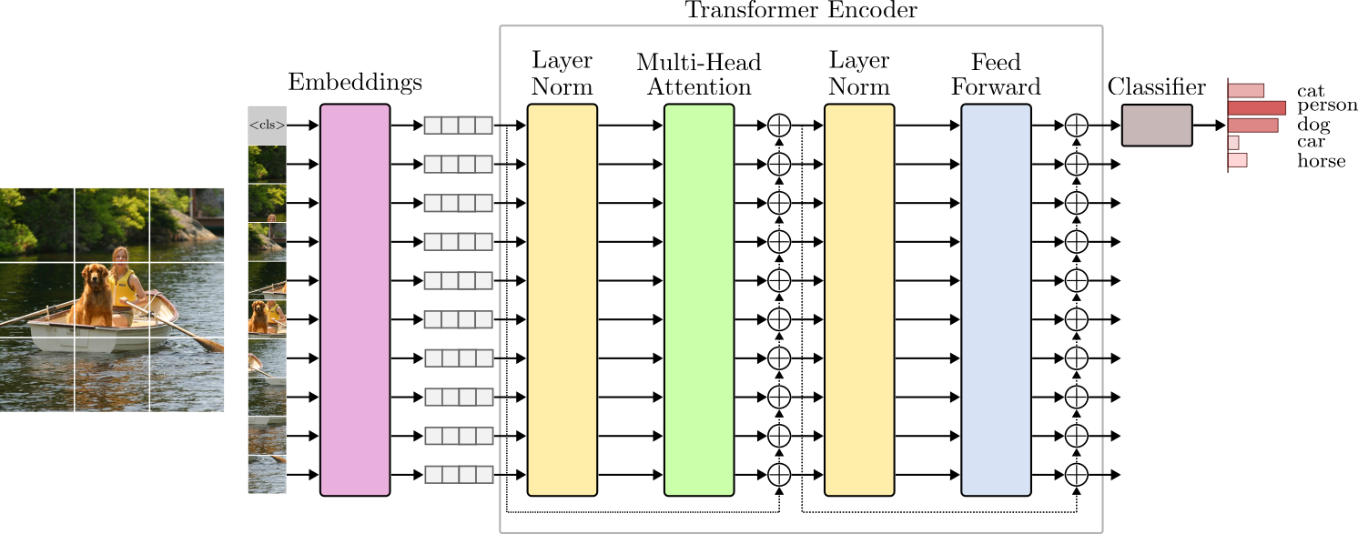
Introduction

Since its proposal in the paper “Attention is all you need” Dosovitskiy, et al. 2015¹, the Transformer architecture has taken deep learning by storm. Initially designed for solving sequence-to-sequence tasks such as machine translation, the Transformer is now everywhere. From natural language processing (NLP) to audio, video, and image applications, the Transformer seems to unify all perception tasks into a single architecture.

The success of the Transformer cannot be pinpointed to a single feature or technique. Indeed, the Transformer combines ideas from different research into an elegant design. Such a design has stood the test of time. Despite many research proposals to “improve” the original architecture, it has remained nearly the same since its introduction.

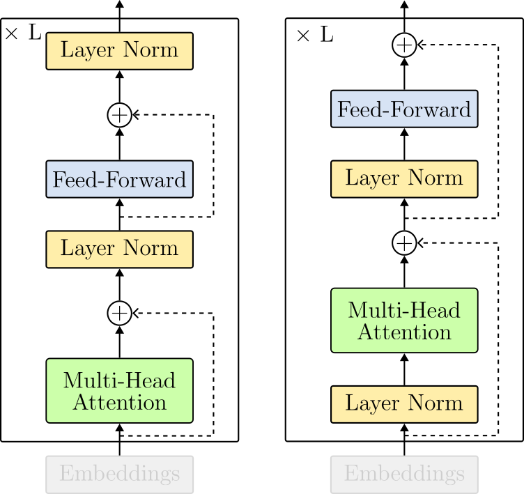
In this article, we will implement the Transformer architecture described in Figure 1 from scratch.

However, we will not focus on NLP applications. Instead, we will implement and develop intuitions on the Transformer from the computer vision perspective.

Because the Transformer was designed to handle NLP tasks, the intuitive understanding of its building blocks is more straightforward when dealing with text. Nevertheless, many of the same intuitions that apply to NLP also translate well to image data, and we will make the bridge between NLP and vision as much as possible.

Before we proceed, check out the complete implementation of the vision Transformer in PyTorch.

This will be a long one, so sit tight and enjoy.

From Tokens to Embeddings

The first layer of the Transformer is the Embeddings layer. This layer maps tokens in the input space to low-dimensional vectors called embeddings.

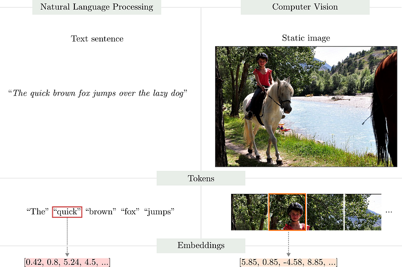
In NLP, the concept of a sequence of elements, or tokens, is natural. In a sentence like,

we can see that,

1. the word ordering matters, and
2. the meaning of words depends on the context they appear.

In NLP, one of the first data processing steps to train a Transformer is converting the training text data into tokens. This process is called tokenization.

There are many ways to do that. The most popular are:

1. Character-based tokenization,
2. Word-based tokenization,
3. Subword-based tokenization.

As the name suggests, when doing character-based tokenization, we split the text data into characters, and each unique symbol is a token.

This tokenization strategy has some advantages. First, the vocabulary size (the number of unique tokens) tends to be small. For instance, the total vocabulary size in English would be only 256 tokens. However, breaking sentences into characters has the effect of making the input context quite large.

We can decide to tokenize text by words.

In this case, the vocabulary size will be very large. To have an idea, the English language can have nearly 170000 unique words. On the plus side, the input context will be smaller if compared to character-based tokenizers.

In addition, a middle-ground strategy called subword tokenization was proposed to solve the problems of character and word-based tokenizers. The idea behind subword tokenization is to break uncommon (or rare) words into smaller subwords. There are many algorithms for subword tokenization. The most popular are WordPiece, used to train BERT, and Byte-Pair Encoding, used to train GPT.

If we employ a word-based tokenizer in the sentence above, we get nine unique tokens. More importantly, we can see that each token interacts differently with the other tokens in the sentence. For instance, the tokens “quick” and “brown” refer to the token “fox” while the token “lazy” refers to “dog”. Moreover, the token “jumps” actually refers to both tokens “fox” and “dog” as – the fox is jumping over the dog.

In computer vision, the notion of a sequence is unclear if we are working with static images. Here, the analogy to text processing is not the best. To understand written text, humans follow pre-defined rules, such as reading from left to right and top to bottom. However, when looking at an image, we do not follow any specific order to understand its content. In other words, to understand that the fox is jumping over the dog in the image below, there is no particular order to look at.

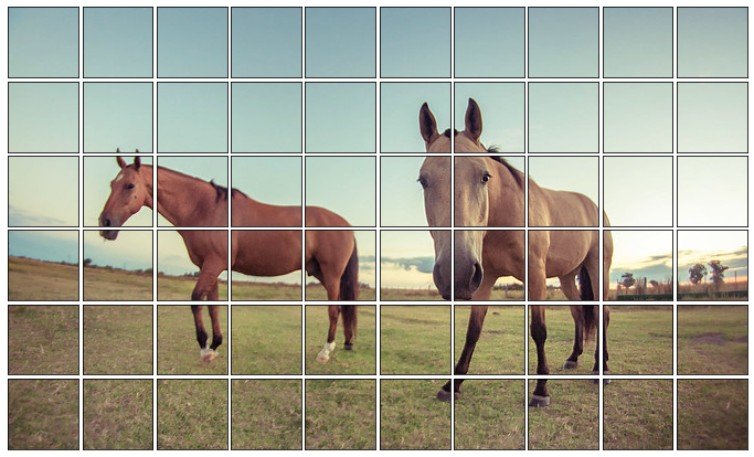
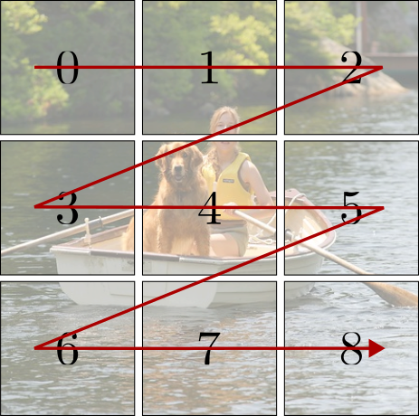
In practice, one way to establish the concept of a sequence on a static image is to extract several patches in a pre-defined order, such as the raster order, refer to Figure 4. In the raster order, patches are extracted from left to right and top to bottom. However, note that this is an arbitrary choice and should be taken with a grain of salt.

Similar to NLP, we can think of these patches/crops as tokens – the elements of the sequence. In NLP, tokens are mapped to low-dimensional vectors called word embeddings. Similarly, image patches are mapped to low-dimensional vectors called visual embeddings.

There is one important difference between the two modalities. When working with text, we can establish a finite dictionary of tokens. The language does not matter. It can be English, Chinese, or any other. The vocabulary size might be large but will always be finite. Hence, we can perform a one-to-one mapping between tokens and embedding vectors. With images, however, that is not possible. Different from text, images live in a continuous higher dimensional space. Therefore, we cannot map a patch/token to a pred-defined embedding. Instead, we must learn a projection matrix $W_e$ to map a high-dimensional image patch (token) in the pixel space to a low-dimensional visual embedding.

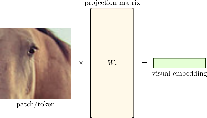
The same projection matrix, $W_e$, is used to project all the patches into low-dimensional embeddings. In the example above, we cropped 60 non-overlapping patches (tokens) from the input image. If we define an embedding dimension of 128, we will have 60 visual embeddings arranged as a 3-dimensional tensor of shape $(1 \times 60 \times 128)$ after projection.

Ordering Matters

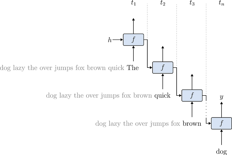
Before the popularization of the Transformer, Recurrent Neural Networks (RNNs) were the go-to option for training deep models on sequential data such as text. To train an RNN, the sequence of tokens is processed one by one, respecting their ordering.

Training RNNs is notoriously tricky. To begin, they are hard to parallelize. Since tokens are processed sequentially, there is a natural dependency between the sequence elements. Also, they require careful tuning to avoid collapse. In short, longer sequences produce undesirable effects in the gradients that optimize the models’ parameters. As a result, RNNs struggle to learn patterns from longer sequences. Figure 7 quickly summarizes the architecture of a Recurrent model.

Unlike RNNs, one of the main features of the Transformer architecture is the ability to process the input all at once. In other words, with Transformers, we can feed the sequence of tokens simultaneously and process them in parallel. As a result, training Transformers is significantly faster because it perfectly suits the GPU data processing model.

You may compare Figures 7 and 8 to see the difference between RNNs and Transformers regarding data ingestion and processing.

However, processing the entire sequence in parallel means that tokens have no dependencies. While this is paramount for processing speed, we lose an essential piece of information – the tokens’ relative positions.

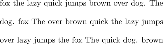
Let’s think about it. If the order in which the Transformer processes the tokens of a sequence does not matter, it means the tokens have no dependencies among themselves. For NLP applications, this may be catastrophic. After all, how could we (or the machine) understand a sentence without ordering among the words? Take a look at Figure 8 to see what happens if we randomize the words of a sentence.

For this reason, before feeding the token embeddings to the Transformer, we need to add the position information to the embeddings. There are many ways of doing this. One of the most popular is to allow the model to learn the positions by itself. The idea is simple. Instead of manually specifying the ordering of each token (which is a valid option), the model will learn positional embedding vectors from the data. 

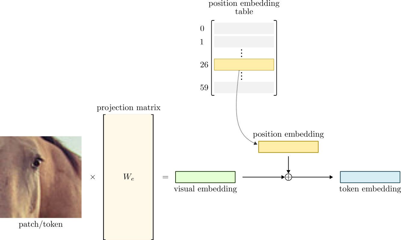
Consider the image in Figure 4 as an example. Each one of the 60 patches is considered a different position. Thus, we need to train additional 60 positional embeddings, one for each crop’s position. Then, we add the position and visual embeddings together to obtain our final, position-aware token embedding. Note that the visual and position embeddings must have the same dimensions. Figure 9 summarizes this process.

Now, let’s code up our Embeddings layer.

The Embeddings Layer in PyTorch

The Embedding layer should contain both logic:

1. the projection of patches into visual embeddings, and 
2. the position embeddings. 

The logic of cropping and projecting an image patch to a low-dimensional embedding vector can be done with convolutions. We just need to set up the kernel_size, which represents the patch size, and the stride, which controls the step between the patches. For example, if we set the kernel_size and the stride to 64, each convolution will operate on non-overlapping image patches of size $64 \times 64$. The code below implements the layer Embeddings().

Since we know the number of positions in advance, we can build an embedding table and select the correct embedding based on the patches’ position. Remember, the patches are extracted following the raster order, Figure 10. Thus, we establish the patches’ position from left to right and top to bottom.

We use torch.arange() to compute the tokens’ positional indices. Then, we use these indices to select the correct embedding vector from the position embedding look-up table.

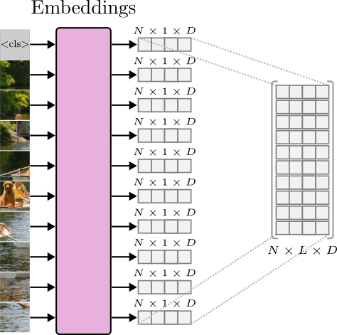
Then, we combine the visual and positional embeddings and normalize the resulting token embedding. Figure 11 visually displays the inner workings of the Embedding layer.

In summary,

1. The Embeddings() layer receives a batch of images of shape $(N \times 3 \times H \times W)$, where $N$ is the batch size, 3 indicates an RGB image, and $H$ and $W$ represents the height and width of the image.
2. Each image in the batch is broken into a series of small patches, and each patch is converted to a low-dimensional embedding. This process is done using the convolutional operation.
3. The layer additionally trains a positional embedding table. Each embedding in the table holds the position information of each token in the sequence.
4. The position and visual embeddings are combined using summation.
5. For each token, the Embeddings() layer will produce a low-dimensional tensor of shape $(N \times 1 \times D)$, where $D$ is the dimensionality of the embedding vector. The output tensor is usually viewed as a stacked tensor of shape $(N \times L \times D)$ where $L$ is the sequence length.

To better understand how Transformers was trained on a large scale, the original vision Transformer was trained with a batch size of 4096 images, each with a shape of $(3 \times 224 \times 224)$. They experimented with different patch sizes, such as $(16 \times 16)$ and $(14 \times 14)$, to extract the tokens. For patch sizes of dimensions $(16 \times 16)$, an RGB $(224 \times 224)$ image was broken down into 196 patches/tokens. Each token was projected to a low-dimensional embedding of size 768. As a result, the Embeddings layer produced an input tensor of shape $(4096 \times 196 \times 768)$. That was the input to the Transformer encoder.

Now, we can jump into the next and very important processing block of the Transformer - the Multi-Head Attention layer.

Looking at the Surroundings - The Multi-Head Attention Layer

The Multi-Head Attention layer is where the tokens interact with one another. This layer allows the neural net to learn patterns and relationships across tokens. 

Attention is a technique that allows a learning algorithm to learn semantic dependencies or affinities among elements of a sequence. In other words, a token is encouraged to pay attention to other elements based on how similar they are.

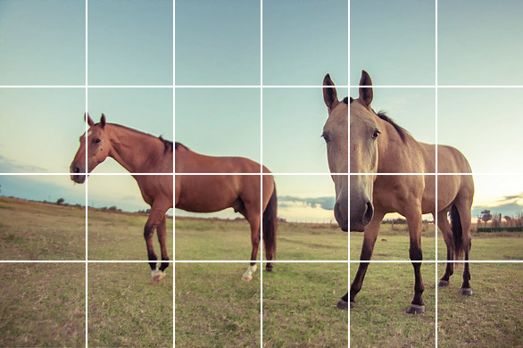
To get a strong intuition of the attention algorithm, let’s review our input image from before.

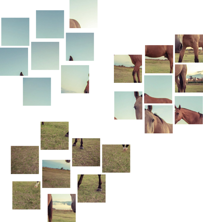
Before we go further, let us examine or “pay attention” to some interesting characteristics of this image. One of the first things to observe is its level of complexity. Note how one could segment the image based on regions similar in structure and textural characteristics. The regions depicting the sky, the grass, and the horses encode similar-looking content. For example, the sky looks extremely similar throughout its course. The same goes for the ground grass, the horses, etc. But at the same time, these regions differ a lot from each other. This property is called spacial locality and is one of the most interesting characteristics of image data. With spacial locality, we can assume that pixels nearby are very similar in terms of visual similarity. In fact, the convolution operator is built on top of this inductive bias. Indeed, the Vision Transformer explores this property when extracting small patches and treating them as tokens. However, some similar regions might extend large portions of an image. In other words, similarities are not only local!

Now, let’s crop 25 non-overlapping patches and tokenize them. Here, we deliberately increased the patch size for understanding purposes.

If we look at these crops, we will notice the same pattern. Some patches from the sky look almost indistinguishable from one another. The same applies to patches including the horse and the ones including the grass. However, if we compare the patches containing mostly grass with patches from the sky, we could argue that they come from different images, given how different they are. Indeed, we could cluster these patches in three or four groups based only on texture similarity.

As we saw, the Transformer receives token embeddings and processes them independently in parallel. But we don’t want to forward these tokens independently through the network all the way to the classification layer. If we did that, the network would not be able to learn relationships among tokens.

As we argued before, to understand a text sentence, we need to understand how the words in the sentence relate. In our text example, the relationship between the words “fox” and “dog” is important to understand the sentence’s meaning. Therefore, to learn a useful representation of text, the network must learn the relationship between the words in the sentence. 

We can draw similar intuitions when working with images. Just like the tokens “fox” and “jumps” share a semantic relationship, some visual tokens relate to one another. This relationship may be based on texture (all the similar patches from the sky) or structure (a patch of the horse’s right ear and another one with the horse’s left ear). Thus, to learn such relationships, we need a way to make the network learn patterns across the tokens of the sequence.

The attention algorithm allows the model to look at the neighboring tokens and decide which patches encode similar-looking information. This way, patches with high affinity could be combined into a contextualized representation that encodes long-range visual similarities of the input image.

Attention as a Dictionary Lookup task

One way to understand the attention algorithm is through the lens of a dictionary look-up search. In Python, we can store key-value pairs in a dictionary object that implements a hash table. To build a dictionary, we associate a key with a value, as in the example below.

If we want to retrieve a value from the dictionary, we check if the query matches one of the keys. If there is a match, we receive the corresponding value as a result. If there is no match between the query and keys, we may get an exception telling us the query is not in the dictionary.

Note that using Python’s dictionary, we either get a match between the query and keys or we don’t. Attention works in a similar way.  The one important difference is that attention allows for soft matches.

In other words, to get a value from the dictionary, we don’t need to match exactly one of its keys. If a query is similar to, but not exactly equal to, a key, we get a value proportional to that measure.

In the Python example above, query and keys are strings. In Attention, query, keys, and values are high-dimensional vectors. In Python, we compare the hashes from the query and key and only return the value if they match. To do something similar in Attention, we need a way to measure the similarity between two vectors. One way is by computing their dot product. With the dot product, if two vectors are similar, the dot product will return a positive value. If the two vectors are not alike, the result might be zero or negative.

Following this reasoning, we can adapt the code example above to resemble the attention algorithm.

In the example above, we have a dictionary where keys and values are vectors. Well, the keys are actually Python Tuples because dictionaries only support hashable types as keys, but that is not important here. In the same way, we define a query vector and search for it in the dictionary. Since our query matches one of the keys, we get a value vector. Everything looks fine so far.

But remember, Python’s dictionary will only return a value if an exact match exists! To visualize this, what if we define a new query as:

Now, we got an exception telling us there was no match between our query and the keys. However, note how the query vector is extremely similar to one of the keys, but this similarity was not taken into consideration because the dictionary only supports exact matches.

Attention as a Soft Selection Mechanism 

In attention, values are not selected only based on exact matches. Instead, the algorithm combines values based on the similarity strength between the query and keys.

To do this, we need a way to measure the similarity between two vectors. If we use the dot product to compute similarities between our query and keys, we will get the following results.

Note how the dot product between the query and the third key vector is the largest. This aligns with the fact that the query tensor is similar to the third key tensor.

These similarities will be used to combine the values. But in their current state, it is unclear how they can be used to select the values from the dictionary accordingly. Thus, the next step is to normalize the similarity scores to more meaningful quantities. Intuitively, if we normalize these values to be between 0 and 1 and sum to 1, we can use them to compute weighted averages of the values.

We can achieve this normalization objective with the softmax function.

Now we can interpret the attention mechanism from a soft assignment perspective where the query vector is nearly 0% similar to the first key vector, 0.002% similar to the second, 97.5% similar to the third, and 2.4% similar to the fourth key vector. Hence, we can combine the values tensors so that the result will have 97.5% of the third value tensor, 2.4% of the fourth value tensor, and so on. This weighted combination is done by matrix multiplying the weights tensor by the values tensor, as follows.

Note how the resulting tensor is much more similar to the third row of the values tensor than the others. That is attention!

Self-Attention For Vision Transformers

Now that we understand how the attention algorithm works, let’s implement it for sequential data.

As we saw, after tokenization, the input to the attention layer will be a tensor of shape $(N \times L \times D)$, where $N$ is the batch size, $L$ is the sequence length, and $D$ is the dimension of the embedding vector. If we project the patches to a 256-dimensional space, the example image above would produce an input tensor of shape $(1 \times 25 \times 256)$. In other words, each of the 25 patches of the sequence is represented by a 256-dimensional vector.

The way the self-attention layer performs token interaction is by measuring similarity among the tokens of the same sequence. For now, let’s define query and keys as identical vectors equal to the input token embeddings. To perform self-attention, we can compute the dot product between all the embedding vectors simultaneously. Since we have 25 such embeddings, one for each patch, we will obtain a similarity scores tensor of shape $(1 \times 25 \times 25)$. In PyTorch, it looks like this.

Here, we can see that the complexity of the attention algorithm grows quadratic with the sequence length. We can better visualize the time complexity by writing a sequential algorithm to compute the scores.

For each token $i$, we compute the dot product between tokens indexed by $i$ and $j$ for $j=0,1,…,24$. 

Now, if we take a look at the scores matrix, we can see how similar each embedding vector is to all the other ones. If we focus on the first patch (first row of the scores $(25 \times 25)$ similarity tensor), we can see how it relates to the other patches in terms of similarity.

With no surprise, the highest similarity comes when we compare the same patch with itself. However, we can see an interesting pattern here. As expected, similar-looking patches have higher dot product outcomes. On the other hand, patches with fairly different pixel distributions have smaller similarity scores. 

To understand how attention works, we need to change how we interpret these values. Instead of viewing them from a similarity perspective, we can interpret them as weights. From this point of view, each weight represents how much the query vector should focus on or attend to each visual token.

To achieve such an effect, we normalize the similarities to the range of $[0, 1]$ and sum to 1. We can view this as establishing bounds to how much we can attend to each element.

We use the weights to create a new vector as a weighted combination of all the patch embeddings we have. This output vector has a contribution from all the other patch embeddings. And this contribution is proportional to their respective weights. That is, the output vector will have 59.0% of the first embedding, 22% of the second embedding, 16% of the third embedding, and so on.

This way, the output vector will be very similar to the embedding vector from the first image, which is the same patch, which makes sense since that is where the weights tell us to pay more attention. But the output vector also has a relatively high contribution from the other patches representing the sky, which are similar.

This procedure is known as the scale dot product attention, and we can summarize it as follows:

In our current implementation, we defined query, keys, and values to be the same vector. As a result, we got very high similarity scores when comparing tokens from the same patch. Also, note that there is no learning in our current attention algorithm.

We are still working on attention, but we can summarise the scale_dot_product_attention() algorithm in 3 steps.

1. First, compute the similarity scores between queries and keys.
2. Second, normalize the similarity scores to obtain the attentionweights.
3. Third, combine the attention weights with the values tensor to produce weighted combinations based on affinities between the tokens of the sequence.

Now, let’s add some learning to the Attention layer.

The Parameterized Attention Head 

Ideally, we would like the network to decide where to pay attention. To do this, we create different sets of variables representing query, key, and value by projecting the input tensor to different linear spaces. Then, we use these projections to perform comparisons. Intuitively, we reduce the correlation between the same patches by projecting the input tensor to a different space. Since the linear projection is learnable, the model can decide where to pay attention to and to which extent. 

This is the idea of an attention head. In PyTorch, we can write it as follows.

In the forward() method we linearly project the input tensor using three independent linear transformations to produce query, key, and value tensors. Then, we call scale_dot_product_attention() using the projected query, key, and value tensors. 

Ideally, a projection head will learn to focus on specific aspects of similarity between the embeddings. Thus, in practice, we may have multiple heads, and each one is free to pay attention to different aspects of similarities.

We can relate having multiple attention heads to learning multiple convolutional filters in convolutional neural networks (CNNs). In CNNs, each filter may learn a different pattern from the input. One filter might detect edges in the horizontal direction, while others might learn to detect edges diagonally. In the same way, having multiple heads allows the model to pay attention to different aspects of similarity. Take the following image patch as an example.

This patch contains three distinct regions (1) a portion of the grass, (2) a piece of the sky, and (3) a part of the horse. In this scenario, a given attention head might focus on patterns from the textual characteristics of the sky, while other heads may focus on finding similarities regarding the horse’s shape and the grass.

That is it for the attention layer of the vision Transformer. After allowing the token of the sequence to interact and merge based on similarity, the Transformer has a layer to process these contextualized representations–the Feed-Forwad layer is our next topic.

The Feed-Forward Layer

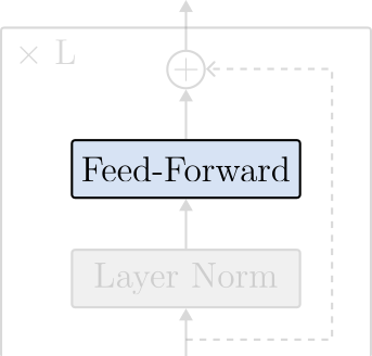
The Feed-Forward or MLP layer is a simple two-layer fully-connected neural network with GELU activations. The layer receives the input tensor of shape $(N \times L \times D)$ from the multi-head attention layer and processes the tokens independently in parallel. Intuitively, we can view the Feed-Forward layer as a processing layer to extract patterns from the contextualized attention vectors. In other words, after being processed in the Attention layer, the token embeddings contain information from the entire sequence – now, they are contextualized embeddings. Therefore, processing them independently strengthens the attention patterns of each token in the sequence.

Coding up this layer is straightforward.

One interesting detail to pay attention to is that we usually use linear layers to process data with shape $(N \times D)$. However, since we are working with sequences, the tensor has has an extra dimension and has a shape of $(N \times L \times D)$. Note that in the first case, the linear layer is applied independently across the elements in the batch. Similarly, in the case of the Transformer, the linear layer is applied independently over the batch and the sequence dimensions.

The Transformer Encoder

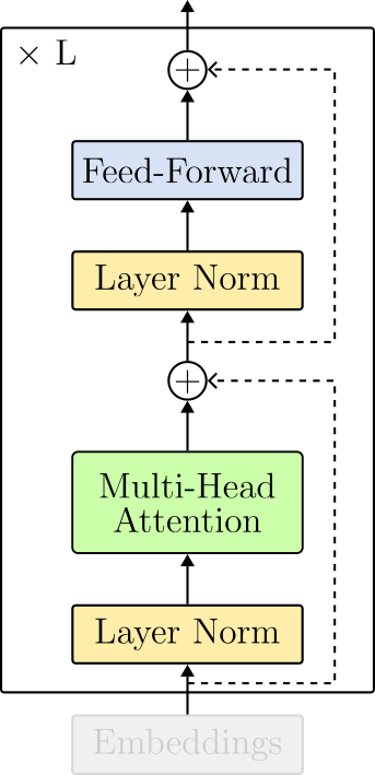
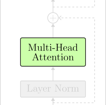
The transformer encoder puts all the pieces together. The block is composed of the following sequence of operations: 

1. Layer Normalization,
2. Multi-Head Attention,
3. Layer Normalization, and
4. Feed-Forward.

Note that the operations are intercalated by residual connections (dotted lines in the Figure above).

We have covered Attention and the Feed-Forward layers. Let’s explore the two missing components: residual connections and layer normalization.

Residual Connections

This brings us to the residual (or skip) connections. Residual connections were introduced in the ResNet paper He, et al. 2016² to avoid the degradation problem when training deep neural networks. Simply put, before residual connections, scaling up neural networks was not just a matter of having more training parameters. In fact, without residual connections, a deep neural network (with more trainable parameters) can perform worse than a neural network with fewer parameters - and that is not because of overfitting. Residual connections allow the gradients to flow without much decimation during training. As a result, we can train very deep models and trade-off more trainable parameters with accuracy.

In practice, a residual block adds the processed tensor back to its original input. In Figure 15, the residual connections are represented as dotted lines.

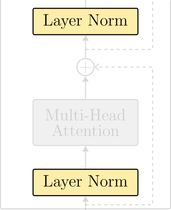
Layer Normalization

Layer normalization is an alternative to one of the most mysterious and problematic layers of modern deep learning – the batch normalization (BN) layer. In batch normalization, tensors processed by a neural network are normalized to resemble a normal distribution with parameterized mean and variances. This normalization occurs in the batch dimension. As a result, a BN layer breaks the independence between input samples.

Another issue with BN layers arrives at inference mode. After training, if we want to use a BN-based model for inference with a single input example, calculating a mean and variance would not be possible. For this reason, it is standard practice to estimate the dataset’s statistics during training. Namely, each BN layer computes running means and variances. to be used in inference mode as normalization parameters for the input tensors.

Layer normalization has the same goal as batch normalization. The only difference is that, instead of normalizing the tensors in the batch dimension, it does it in the dimensions of the features. Consequently, layer normalization does not require running estimates for the dataset’s mean and variances and behaves equally during training and inference.

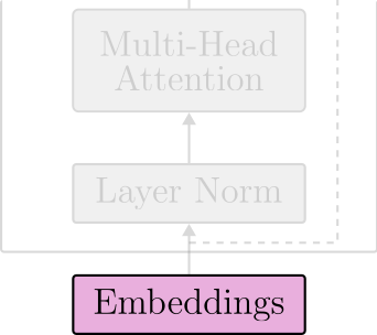
One difference from the original Transformer paper is where layer normalization operates. In the original Transformer, normalization layers were put in between the skip connections. This layout is referred to as post-layer normalization and is not used anymore due to difficulties in training. Instead, the most common arrangement places the layer normalization within the span of the residual connections. This layout is called pre-layer normalization. Figure 15 displays the architectural differences between each option.

The Transformer Encoder Layer in PyTorch

At this point, we can arrange the LayerNorm(), MultiHeadAttention() and the FeedForward() modules to create the TransformerEncoderLayer(). Compare the code below with the architecture design in Figure 15 (right).

To build a vision Transformer, we just need to stack many TransformerEncoderLayer() on top of each other.

Note how the Transformer encoder looks simple. We can summarize it in a few steps.

1. The encoder __init__() function creates the Embeddings() and a list of TransformerEncoderLayer().
2. The forward() method receives a batch of images of shape $(N \times 3 \times H \times W)$, where $H$ and $W$ are the spatial dimensions of the images.
3. The batch images are encoded to position-away token embeddings.
4. The embeddings are passed through the encoder layers.
5. The encoder returns a sequence tensor of shape $(N \times L \times D)$.

Now, let’s go over how we can train the vision Transformer to solve vision tasks.

The Classification Layer

There are many ways of training a Transformer encoder. We use it to solve various supervised tasks such as classification, detection, and segmentation. We can use it for feature learning and optimize a self-supervised objective on unlabeled data. Another option is to take a Transformer encoder trained in a large-scale regime and use it to learn a new task on top of its features.

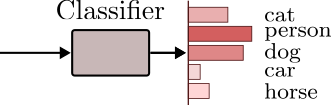
Let’s assume we want to train a classification model. In this case, we can append a new classification head to the Transformer encoder and train the entire model using a classification loss such as the cross-entropy.

However, note that the encoder receives a sequence as input and outputs a sequence tensor of shape of $(N \times L \times D)$. We need to take this sequence tensor and learn a mapping function to a pre-defined number of classes. However, how can we achieve this objective with this sequence tensor?

One option is to average the output tensor at the sequence dimension. This would give us a tensor of shape $(N \times D$) that we could easily be the input to a softmax layer.

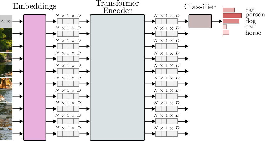
Another popular option is learning a token embedding designed to represent the entire sequence (image). Indeed, if you look at the PyTorch code for the Embedding layer from before, you will see an additional embedding called class_token that stands for classification token and capture this idea.

The class_token embedding is appended to the patch projections as its first component. This is analogous to adding a <CLS> token at the beginning of a tokenized sentence in NLP. Adding the class_token will increase the sequence length by one. As a result, the encoder will produce an output tensor of shape $(N \times L+1 \times D)$. Now, for training and inference, we can take the output tensor of the encoder and discard the rest of the sequence elements and only use the class_token embedding as input to the last classification layer. Figure 16 depicts this idea.

In PyTorch, we can write a TransformerClassifier() module as,

The TransformerClassifier() module builds the TransformerEncoder() and the classification Linear() layer. Note how in the forward() method, we only take the first embedding vector from the encoder output and feed it to the classification layer. This is the class_token embedding vector representing the entire image.

Conclusion

That concludes this introduction to the vision Transformer. I ran a miniature version of the vision Transformer on the CIFAR10 dataset for 100 epochs and obtained nearly 78% on the test set. The complete code can be found here. This performance seems low compared to convolutional architectures with a comparable number of trainable parameters. Indeed, when it comes to vision tasks, the Transformer needs a lot of data to shine! Unlike convolutional models, the Transformer architecture does not explore inductive biases, such as translation invariance. As such, more training data seems to be needed to reach higher performance levels.

Hope you have enjoyed it. Thanks for reading!

Cite as:

@article{
  silva2023visiontransformer,
  title={An Intuitive Introduction to the Vision Transformer},
  author={Silva, Thalles Santos},
  journal={https://sthalles.github.io},
  year={2023}
  url={https://sthalles.github.io/an-intuitive-introduction-to-the-vision-transformer/}
}

References