Matryoshka Representation Learning

Preliminaries

The task of representation learning is to find an optimal code that maintains relevant information from the input. Given a dataset $\mathcal{X}$ and a set of possible labels $\mathcal{Y}$, the goal is to learn a $d$-dimentional representations vector $z \in \mathbb{R}^d$ by learning a mapping function $f(x, \theta): \mathcal{X} \rightarrow \mathbb{R}^d$, where $f$ is a neural network with learnable paraeters $\theta$ such as a Convolutional Neural Network (CNN) (He et al. 2016)¹ or a Transformer (Dosovitskiy et al. 2020)².

This framework works in supervised and unsupervised settings. Given a point observation $x \in \mathcal{X}$, we can get a representation of $x$ by forwarding it through the neural network $f$ such that $z = f(x)$, we omit the parameters for simplicity.

Deep networks designed to learn representations from data are often called encoders.

Learning Representations with Labeled Data

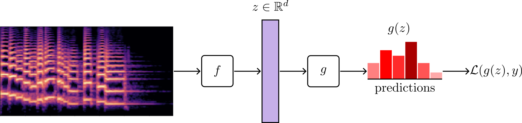
In supervised learning, the encoder $f$ is trained with pairs of inputs and labels \(\left \{ x_i, y_i \right \}_{i=0}^N\) where $N$ is the size of the dataset $\mathcal{X}$. For a classification task over $C$ classes, the encoder is trained by appending a classification layer $g$ with parameters $W \in \mathbb{R}^{d \times C}$ that maps the representations $z \in \mathbb{R}^d$ to one of the possible $C$ classes.

The optimization is usually done using a loss function that takes the predictions and targets such as $\mathcal{L}(g(z), y)$, where a common method is to minimize the negative log-likelihood of the data under the categorical distribution (cross-entropy).

The encoder $f$ learns representations by solving the classification task with $C$ classes. Once trained, we can discard the classifier $g$ and use the encoder to produce low-dimensional vectors as $z = f(x, \theta)$. The pre-trained representations can be used in a variety of ways, such as solving different downstream tasks.

Optionally, one might want to fine-tune (gradually change) the encoder parameters $\theta$ to learn a new downstream task. This technique is called fine-tuning and is one of the most important concepts of deep learning that powers innumerable applications in industry and academia.

Let’s continue with the supervised learning setup throughout the text.

Introduction

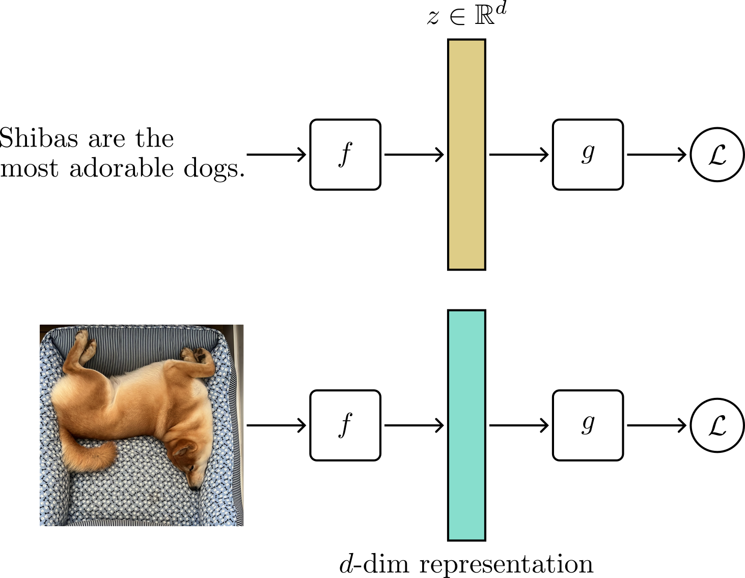
In representation learning, an embedding is a dense vector that encodes semantic information about the input. At a high level, deep neural networks take input (image, text, audio) and output a $d$-dimentional fixed-sized dense vector called a representation or an embedding.

Good representations usually have two characteristics: compactness and generalizability.

Compactness implies that the learned embedding is much smaller than the original input, directly translating to efficient storage and retrieval operations. Consider a ResNet-50 model trained to categorize an image $x$ into one of $C=1000$ possible classes. During training, the ResNet takes as input an RGB image of size $224 \times 224 \times 3$, which requires $602112$ Bytes or $0.602112$ Megabytes to store it, assuming a 32-bit float representation. On the other hand, a ResNet-50 outputs a representation vector of size $2048$, which requires $8192$ Bytes or $0.008192$ Megabytes. Thus, the ResNet-50 provided a code with a $73.5$ compression rate.

Generalizability means that the information encoded on these vectors is not strongly tied to any particular task or dataset. As a result, these features can be used to learn downstream tasks efficiently. In fact, good representations can reduce the training time and the need for large amounts of labeled data while improving the final downstream task performance.

Note that the information within the embedding is diffused across the vector. In other words, we cannot know the meaning of each feature within the embedding nor how they relate to the input.

Representation learning methods usually learn a fixed-sized representation $z \in \mathbb{R}^d$, where the size $d$ is a hyperparameter linked to the choice of neural architecture.

For example,

• The original family of BERT models was trained using two variations of the Transformer architecture. The BASE model produces $768$-dimentional embeddings, and the LARGE produces $1024$-dimentional representations.

• The Original SimCLR self-supervised learning model for computer vision was trained using a ResNet-50 encoder, which produces $2048$-dimentional embeddings.

• The OpenAI text-embedding-ada-002 embedding model outputs $1536$-dimentional representations from text data.

Matryoshka Representation Learning

Matryouska Representations Learning (MRL) (Kusupati et al. 2022)³ is a simple and intuitive idea. Given a representation vector $z \in \mathbb{R}^d$, MRL will pose multiple learning problems at continuous subsets of $z$. Each task optimizes the first $m \in \mathcal{M}$ feature components of $z$ such that the sub-representation $z_{[1:m]}$ is independently trained to be a fully capable representation by itself.

The image below depicts the learning strategy.

Let’s break it down step by step.

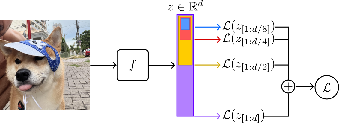
The following sequence of images depicts the MRL optimization process.

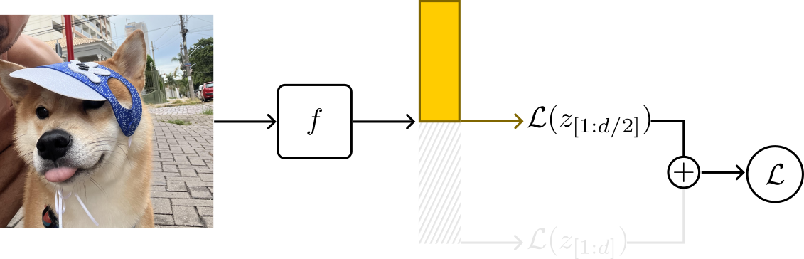
MRL learns a course-to-fine structure by encoding information at multiple granularities of a single embedding vector $z$. Namely, each granularity is composed of the first $m \in \mathcal{M}$ feature components of $z$. Each sub-representation, $z_{[1:m]}$, is optimized independently using a separate classifier and loss function.

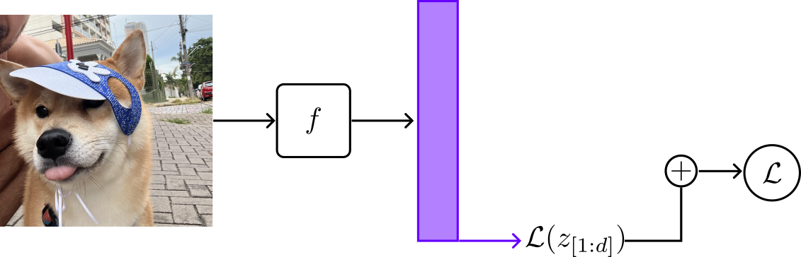
The first loss term looks equal to any other deep learning model. Here, the loss operates over the first $m = d$ feature components of $z$.

Now, things get more interesting. The second term of the loss operates over the first \(m=\frac{d}{2}\) components of $z$. In other words, it operates over the first half feature values of $z$, denoted by $z_{[1:m]}$.

Following, the third and fourth loss terms operate over the first $m=\frac{d}{4}$ and $m=\frac{d}{8}$ components of $z$, respectively.

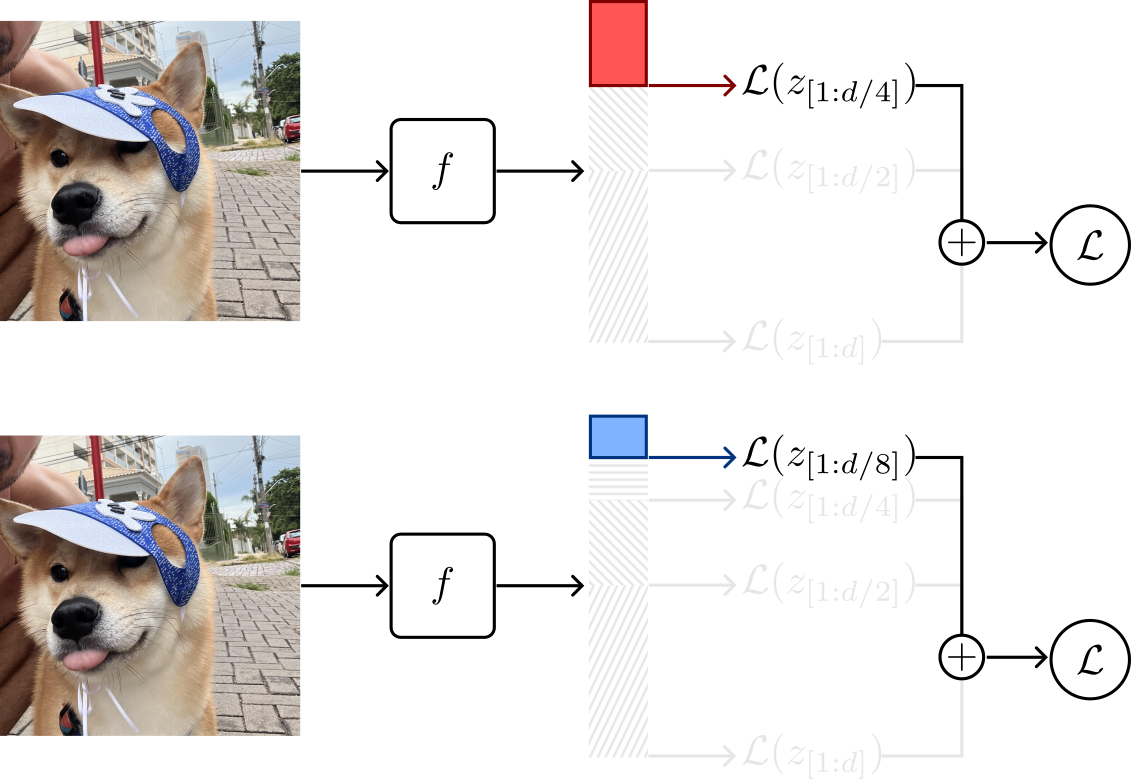
The process of consistently halving the representation vector $z$ and using its first components continues until a minimum capacity, defined as a hyperparameter, is reached.

Formally, from the full representation dimension $d$, we can define $\mathcal{M}$ by progressively halving $d$ until we reach a minimum capacity. For the examples depicted above, we can define \(\mathcal{M} \in \left \{ \frac{d}{8}, \frac{d}{4}, \frac{d}{2}, d\right \}\), where $\frac{1}{8}$ is the minimum representation capacty factor.

Similarly, assuming a representation $z \in \mathbb{R}^{2048}$ from a ResNet-50 encoder, and a minimum capacity factor a $\frac{1}{256}$, we have \(\mathcal{M} \in \left \{ 8, 16, ...,1024,2048 \right \}\).

Then, for each $m \in \mathcal{M}$, we sample a subset containing the first $m$ components of $z$, and indenpendely optimize the sub-representation \(z_{[1:m]}\) using a separate classification head with parameters $\mathbf{W}^{(m)} \in \mathbb{R}^{m \times C}$ and loss function.

Then, we combine the individual loss terms and minimize

$$\mathcal{L}_{MRL} = \frac{1}{N} \sum_i^N \sum_{m \in \mathcal{M}} \mathcal{L} \left ( \mathbf{W}^{(m)} \cdot f(x_i, \theta) \right ).$$

Conclusions

The motivations of MRL representations are efficient storage and fast retrieval, targeted by adaptive deployment use cases. Representations learned by MRL are not particularly better than using a fixed-size embedding training strategy. However, MRL allows us to select different sizes of the representation while trading the minimum accuracy possible.

For example, assuming a full representation vector of ${2048}$-dim in a retrieval-based application, one has the flexibility to choose a smaller representation granularity, such as $z_{[1:16]}$, to achieve efficient storage and faster retrieval. At the same time, one can choose a larger representation granularity to perform tasks that require higher semantic similarity accuracy.

Hope you have enjoyed it. Thanks for reading!

Cite as:

@article{
  silva2023mrl,
  title={Matryoshka Representation Learning},
  author={Silva, Thalles Santos},
  journal={https://sthalles.github.io},
  year={2024}
  url={https://sthalles.github.io/matryoshka-representation-learning/}
}

References