A Visual Guide to Time Series Decomposition Analysis
[machine-learning deep-learning timeseries timeseries-analysis timeseries-decomposition 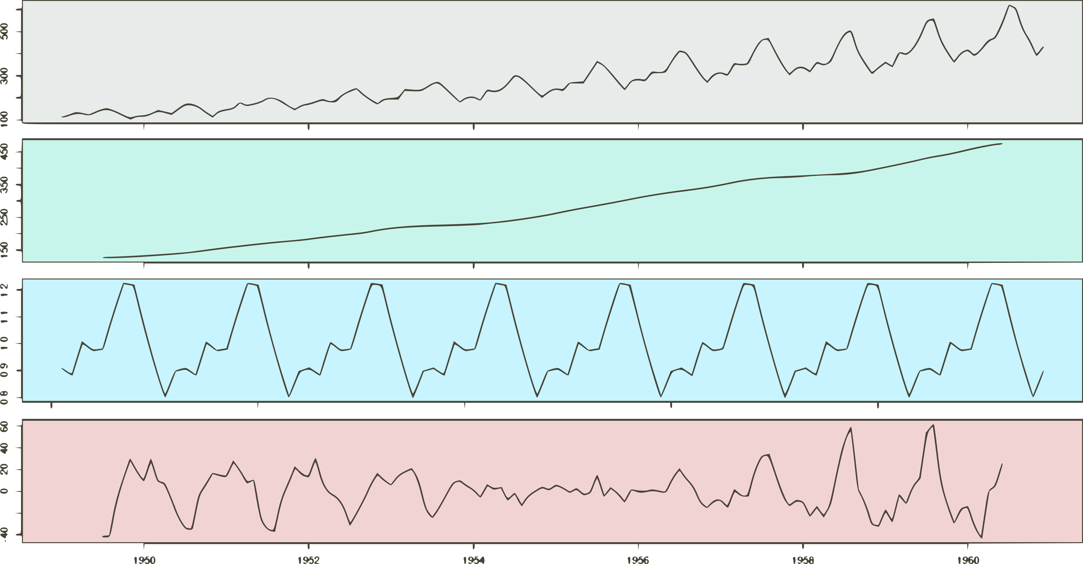
Introduction
Time Series Forecasting is the use of statistical methods to predict future behavior based on a series of past observations. Simply put, we can think of it as a bunch of values collected through time.
Many companies are exploring time series forecasting as a way of making better business decisions. Take a hotel as an example. If the hotel manager has a good idea of how many hosts to expect in the next summer, he/she can use these insights to plan for staff management, budget, or even a facility expansion. Likewise, confident insights for future events can benefit a wide range of industries and problems. From traditional agriculture to on-demand transportation, and more.
Classical forecasting methods like ETS and ARIMA have been around for quite some time. However, the recent machine learning revolution also brought some light to forecasting. The never greater availability of time series data is a pushing factor. Besides, the popularity of deep learning has contributed to the recent increase in interest in the topic.
Moreover, recent algorithms like Facebook Prophet, and CausalImpact are popping up. Some of them use deep learning techniques such as Long Short Term Memory (LSTMs) Networks.
Despite all that, time series forecasting is not an easy problem.
In this piece, we focus our attention on ways of exploring time series data. Our goal is to understand how the various components of a time series behave. This insight is often used when we want to tune or even decide upon which forecasting method to use.
Indeed, choosing the appropriate method is one of the most important decisions an analyst has to make. While experient data scientists have clear intuitions only by looking at a time series plot, time series decomposition is one of the best ways to understand how a time series behave.
Time Series Data
Time series data is a bunch of values collected through time. This kind of data usually exhibits different kinds of patterns. The most common ones are:
- Trend
- Cycles
- Seasonality
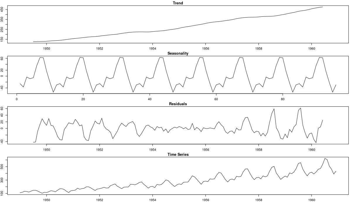
Moreover, depending on the method we choose, we can apply each one of these components differently. A good way to get a feel of how each of these patterns behaves is to break the time series into many distinct components. The idea is that each component represents a specific pattern like trend, cycle, and seasonality.
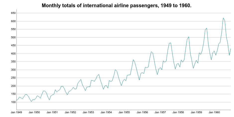
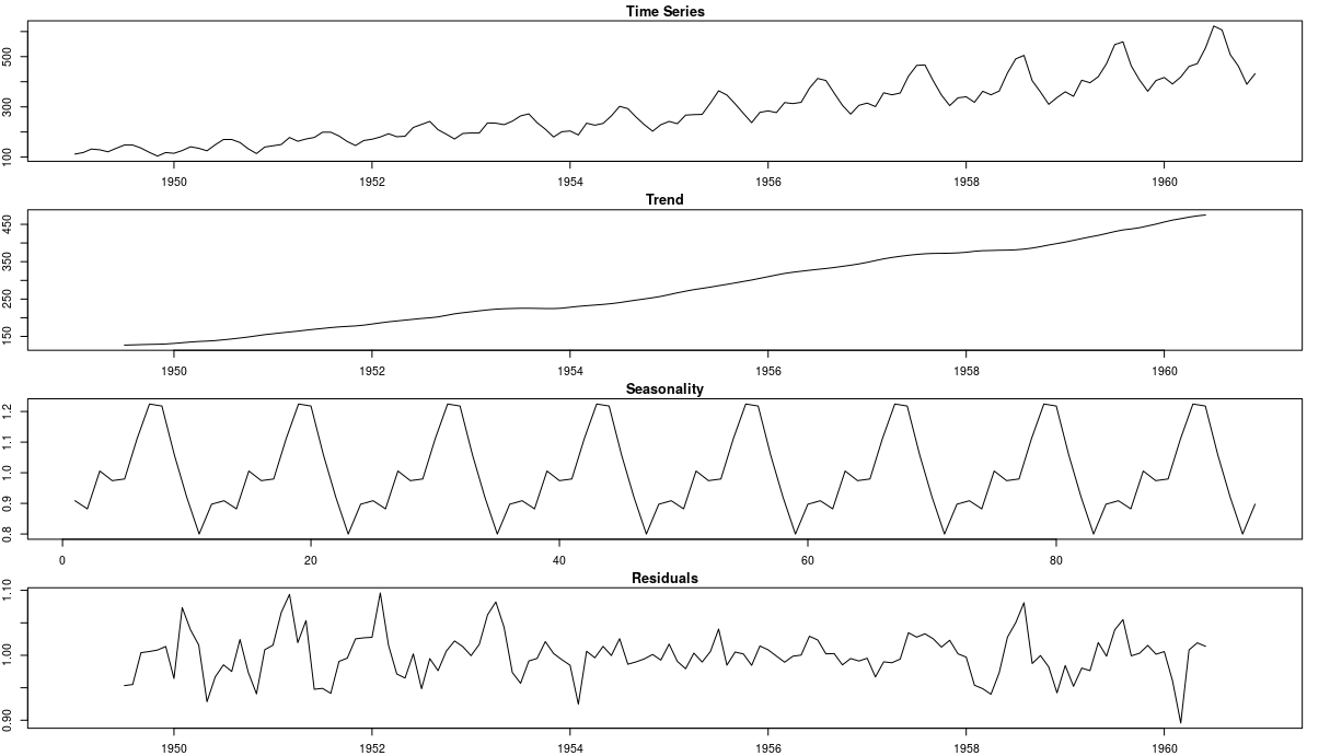
Let’s begin with classical decomposition methods. Below, you can see the International airline passengers time series dataset. It contains 144 monthly spaced observations from 1949 to 1960.
Let’s use it as an example and perform 2 types of decomposition: additive and multiplicative.
Before we begin, a simple additive decomposition assumes that a time series is composed of 3 additive terms.

Likewise, a multiplicative decomposition assumes the terms are combined through multiplication.

Here:
- S represents the Seasonal variation.
- T encodes Trend plus Cycle components.
- R describes the Residuals or the Error component.
- t represents each period.
Additive Decomposition
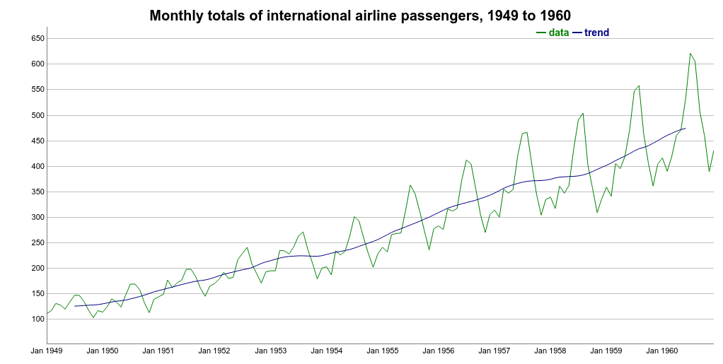
There are many ways to extract the trend component of a time series. Here, we compute it as the centered moving average of the data.
The moving average smoother averages the nearest N periods of each observation. Using R, we can use the ma() function from the forecast package.
One important tip is to define the order parameter equal to the frequency of the time series. In this case, frequency is 12 because the time series contains monthly data. We can see the trend over the original time series below.
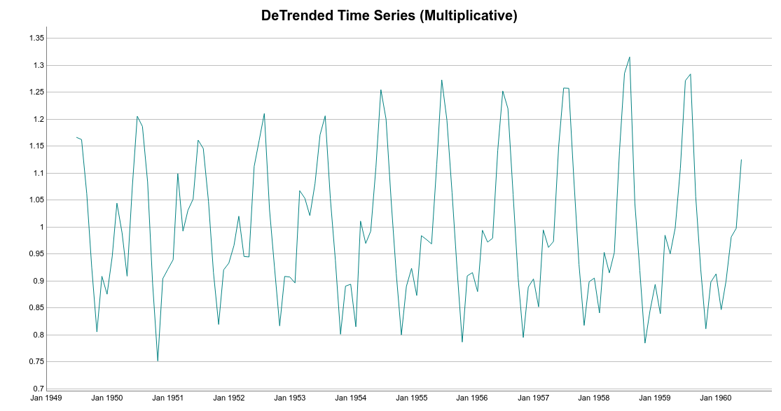
Once we have the trend component, we can use it to remove the trend variations from the original data. In other words, we can DeTrend the time series by subtracting the Trend component from it.

If we plot the DeTrended time series, we are going to see a very interesting pattern. The DeTrended data emphasize the seasonal variations of the time series.
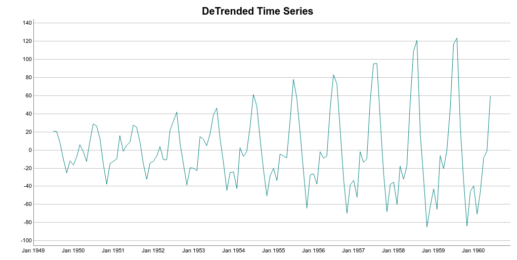
We can see that seasonality occurs regularly. However, its magnitude increases over time. Keep that in mind for now.
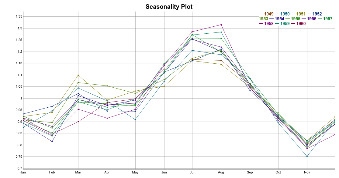
The next step to extract the seasonal component of the data. To do that, we average the monthly DeTrended data based on its period. This can be easier seen using a seasonality plot.
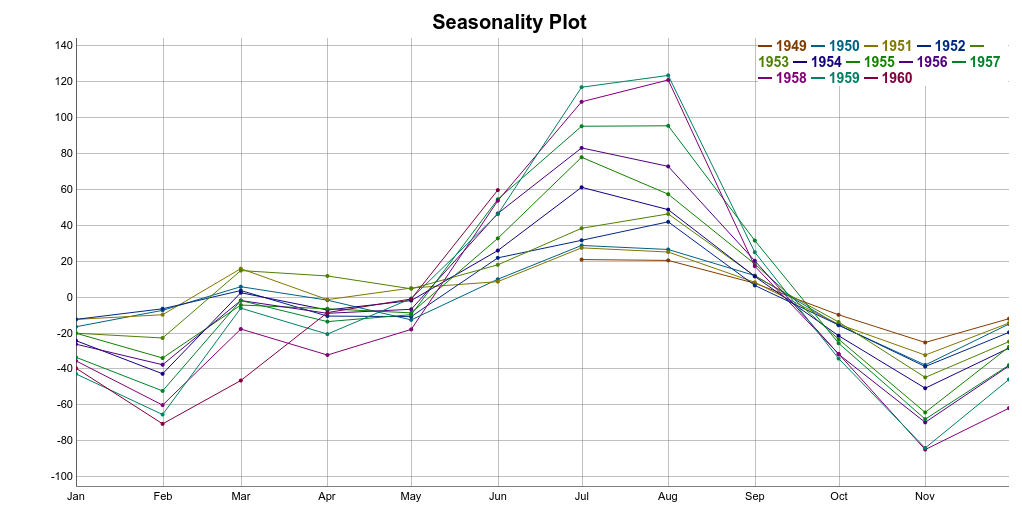
Each horizontal line in the seasonality plot corresponds to a year of data (12 data points). Then, each vertical line groups all data points by its frequency.
In this case, each vertical lines groups data points for each specific month. For instance, here, we are dealing with monthly data i.e. frequency equal 12. Hence, the seasonality value for February is the average of all the DeTrended February values in the time series.
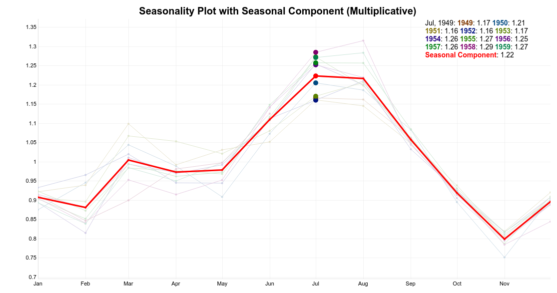
Thus, a simple way to extract the seasonal component is to average the data points for each month. Take a look at the seasonal component highlighted in red on the plot below.
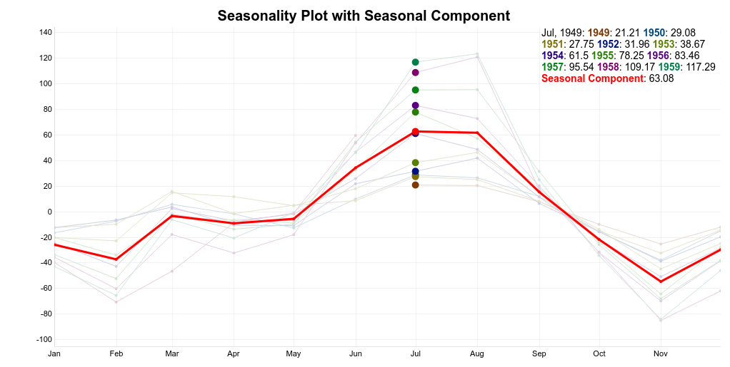
The idea is to use this pattern repeatedly to explain the seasonal variations of the time series.
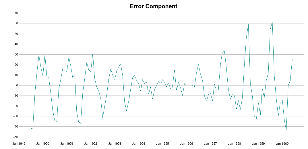
Ideally, trend and seasonality should capture most of the patterns in the time series. Hence, the residuals represent what’s left from the time series, after trend and seasonal have been removed from the original signal.

Also, we want the residuals to be as small as possible.
Finally, we can put it all together in a seasonality plot.
Now, let’s try to reconstruct the time series using the trend and seasonal components.
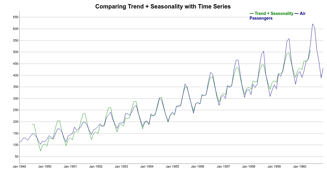
We can see that the reconstructed signal (Trend + Seasonality) follows the increasing pattern of the data. However, it is clear that the seasonal variations are not well represented in this case. There is a discrepancy between the reconstructed and original time series. Note that Trend + Seasonality variations are too wide at the beginning of the series but not wide enough towards the end of the series.
That is because additive decomposition assumes seasonal patterns as periodic. In other words, the seasonal magnitudes are the same every year and they add to the trend.
But if we take a look again at the DeTrend time series plot, we see that it is not true. More specifically, the seasonal variations increase in magnitude over time. Meaning that the number of passengers increased year after year.
Let’s now explore a multiplicative decomposition.
Multiplicative Decomposition
To perform multiplicative decomposition, we do not need to change the way we compute the trend. It still is the centered moving average of the data.
However, to DeTrend the time series, instead of subtracting the trend from the time series we divide it.

Note the difference between the DeTrended data for additive and multiplicative methods. For additive decomposition, the DeTrended data is centered at 0. That is because adding zero makes no change to the trend.
On the other hand, for the multiplicative case, the DeTrended data is centered at 1. That follows because multiplying the trend by 1 has no effect to it as well.
Following similar reasoning, we can find seasonal and error components.

Take a look at the complete multiplicative decomposition plot below. Since it is a multiplicative model, seasonality and residuals are both centered at 1 (instead of 0).
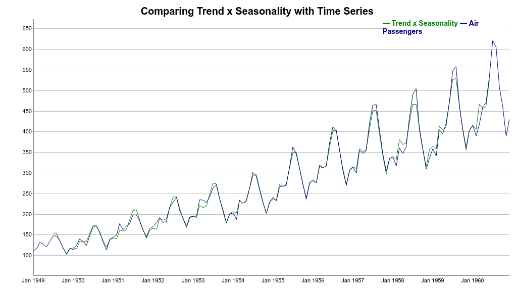
Now, we can try to reconstruct the time series using the Trend and Seasonal components. It is clear how the multiplicative model better explains the variations of the original time series. Here, instead of thinking of the seasonal component as adding to the trend, the seasonal component multiplies the trend.
Note how the seasonal swings follow the ups and downs of the original series. Also, if we compare additive and multiplicative residuals, we can see that the later is much smaller. As a result, a multiplicative model (Trend x Seasonality) fits the original data much closer.
Conclusion
Analyzing a Time Series Decomposition Plot is one of the best ways to figure out how each of the time series components behave.
When seasonal variations remain constant and periodic, additive methods are the way to go. On the other hand, if seasonal swings change over time, a multiplicative method is recommended.
It is important to note that simple decomposition methods have some drawbacks. Here, I highlight two of them.
First, using a moving average to estimate the Trend + Cycle component has some disadvantages. Specifically, this method creates missing values for the first few and last values of the series. For monthly data (frequency equal 12), we will not have estimates for the first and last 6 months. That is depicted on the Trend figure above.
Also, the seasonal pattern estimates are assumed to repeat every year. This can be a problem for longer series where the patterns might change. You can see this assumption on both decomposition plots. Note how the additive and multiplicative seasonal patterns repeat over time. There are more robust methods like Seasonal and Trend decomposition using Loess - STL - that addresses some of these problems.
Thanks for reading!
Cite as:
@article{
  silva2019visualtimeseries,
  title={A Visual Guide to Time Series Decomposition Analysis},
  author={Silva, Thalles Santos},
  journal={https://sthalles.github.io},
  year={2019}
  url={https://sthalles.github.io/a-visual-guide-to-time-series-decomposition/}
}