Deeplab Image Semantic Segmentation Network

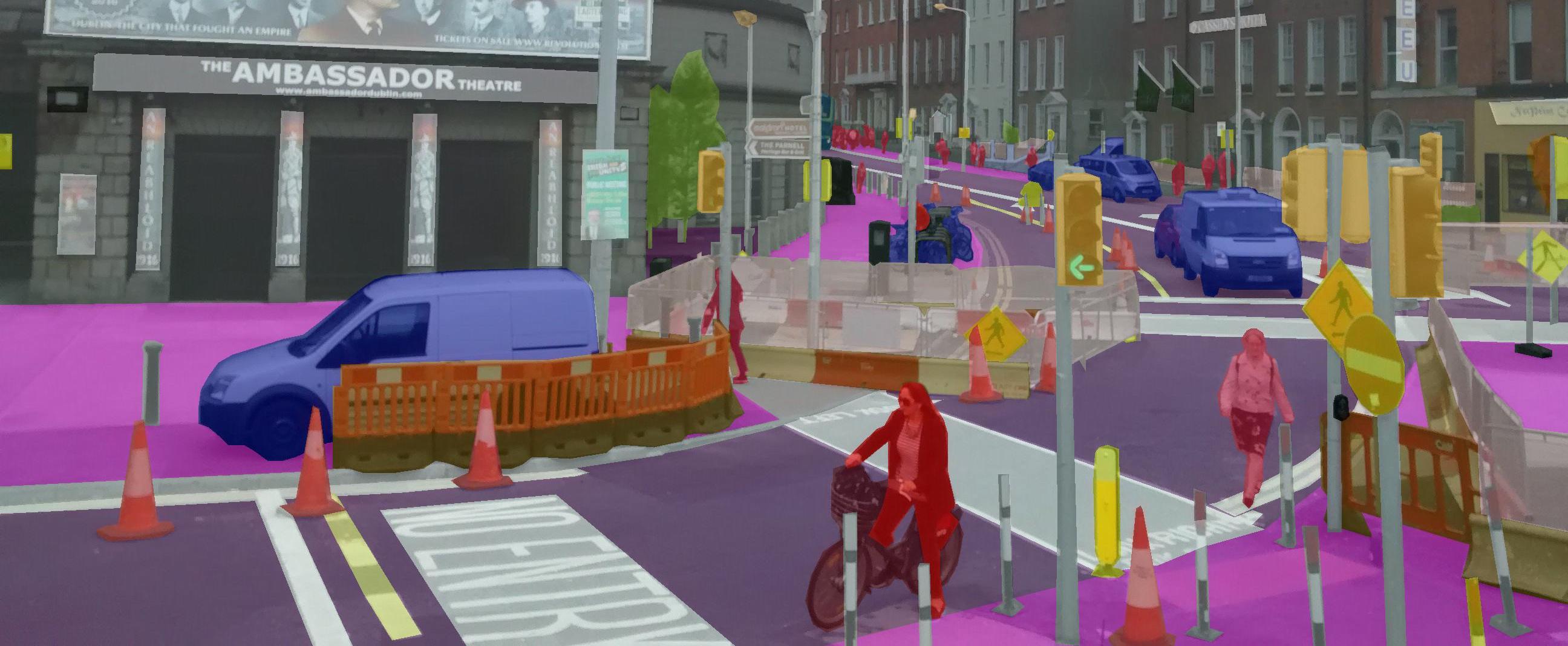
Introduction

Deep Convolution Neural Networks (DCNNs) have achieved remarkable success in various Computer Vision applications. Like others, the task of semantic segmentation is not an exception to this trend.

This piece provides an introduction to Semantic Segmentation with a hands-on TensorFlow implementation. We go over one of the most relevant papers on Semantic Segmentation of general objects - Deeplab_v3. You can clone the notebook for this post here.

Semantic Segmentation

Regular image classification DCNNs have similar structure. These models take images as input and output a single value representing the category of that image.

Usually, classification DCNNs have four main operations. Convolutions, activation function, pooling, and fully-connected layers. Passing an image through a series of these operations outputs a feature vector containing the probabilities for each class label. Note that in this setup, we categorize an image as a whole. That is, we assign a single label to an entire image.

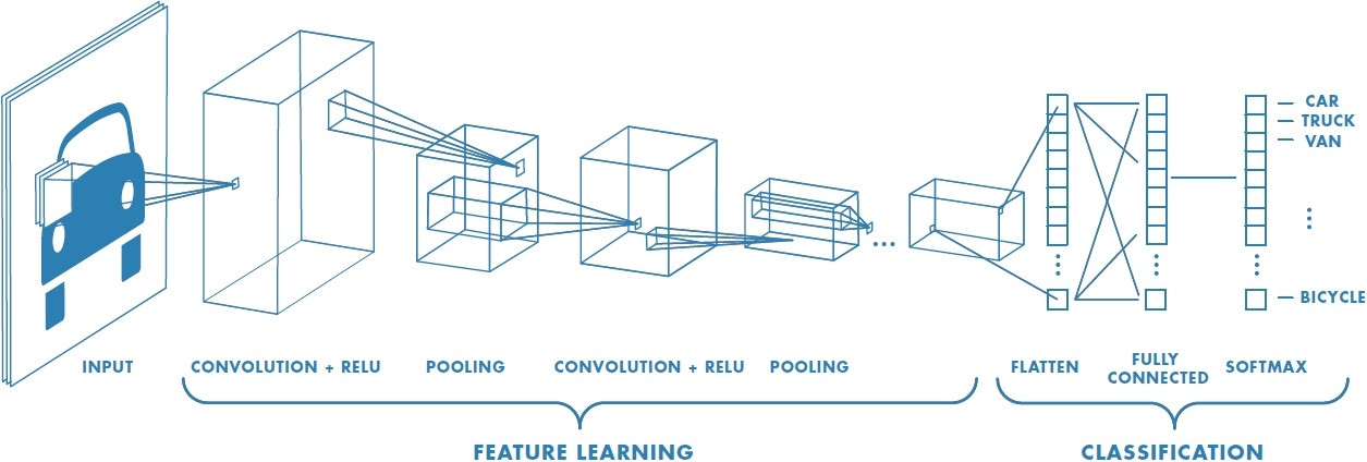
Image credits: Convolutional Neural Network MathWorks.

Different from image classification, in semantic segmentation we want to make decisions for every pixel in an image. So, for each pixel, the model needs to classify it as one of the pre-determined classes. Put another way, semantic segmentation means understanding images at a pixel level.

Keep in mind that semantic segmentation doesn’t differentiate between object instances. Here, we try to assign an individual label to each pixel of a digital image. Thus, if we have two objects of the same class, they end up having the same category label. Instance Segmentation is the class of problems that differentiate instances of the same class.

Yet, regular DCNNs such as the AlexNet and VGG aren’t suitable for dense prediction tasks. First, these models contain many layers designed to reduce the spatial dimensions of the input features. As a consequence, these layers end up producing highly decimated feature vectors that lack sharp details. Second, fully-connected layers have fixed sizes and loose spatial information during computation.

As an example, instead of having pooling and fully-connected layers, imagine passing an image through a series of convolutions. We can set each convolution to have stride of 1 and “SAME” padding. Doing this, each convolution preserves the spatial dimensions of its input. We can stack a bunch of these convolutions and have a segmentation model.

This model could output a probability tensor with shape [W,H,C], where W and H represent the Width and Height. And C the number of class labels. Applying the argmax function (on the third axis) gives us a tensor shape of [W,H,1]. After, we compute the cross-entropy loss between each pixel of the ground-truth images and our predictions. In the end, we average that value and train the network using back prop.

There is one problem with this approach though. As we mentioned, using convolutions with stride 1 and “SAME” padding preserves the input dimensions. However, doing that would make the model super expensive in both ways. Memory consumption and computation complexity.

To ease that problem, segmentation networks usually have three main components. Convolutions, downsampling, and upsampling layers.

There are two common ways to do downsampling in neural nets. By using convolution striding or regular pooling operations. In general, downsampling has one goal. To reduce the spatial dimensions of given feature maps. For that reason, downsampling allows us to perform deeper convolutions without much memory concerns. Yet, they do it in detriment of losing some features in the process.

Also, note that the first part of this architecture looks a lot like usual classification DCNNs. With one exception, they do not put in place fully-connected layers.

After the first part, we have a feature vector with shape [w,h,d] where w, h and d are the width, height and depth of the feature tensor. Note that the spatial dimensions of this compressed vector are smaller (yet denser) than the original input.

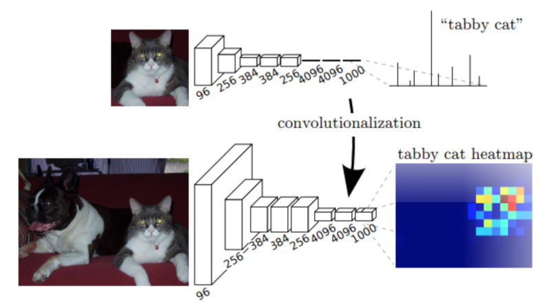
Image credits: Fully Convolutional Networks for Semantic Segmentation.

At this point, regular classification DCNNs would output a dense (non-spatial) vector containing probabilities for each class label. Instead, we feed this compressed feature vector to a series of upsampling layers. These layers work on reconstructing the output of the first part of the network. The goal is to increase the spatial resolution so the output vector has the same dimensions as the input.

Usually, upsampling layers are based on strided transpose convolutions. These functions go from deep and narrow layers to wider and shallower ones. Here, we use transpose convolutions to increase feature vectors dimension to the desired value.

In most papers, these two components of a segmentation network are called: encoder and decoder. In short, the first, “encodes” its information into a compressed vector used to represent its input. The second (the decoder) works on reconstructing this signal to the desired outcome.

There are many network implementations based on encoder-decoder architectures. FCNs, SegNet and UNet are some of the most popular ones. As a result, we have seen many successful segmentation models in a variety of fields.

Model Architecture

Different from most encoder-decoder designs, Deeplab offers a different approach to semantic segmentation. It presents an architecture for controlling signal decimation and learning multi-scale contextual features.

Image credits: Rethinking Atrous Convolution for Semantic Image Segmentation.

Deeplab uses an ImageNet pre-trained ResNet as its main feature extractor network. However, it proposes a new Residual block for multi-scale feature learning. Instead of regular convolutions, the last ResNet block uses atrous convolutions. Also, each convolution (within this new block) uses different dilation rates to capture multi-scale context.

Additionally, on top of this new block, it uses Atrous Spatial Pyramid Pooling (ASPP). ASPP uses dilated convolutions with different rates as an attempt of classifying regions of an arbitrary scale.

To understand the deeplab architecture, we need to focus on three components. (i) The ResNet architecture, (ii) atrous convolutions and (iii) Atrous Spatial Pyramid Pooling (ASPP). Let’s go over each one of them.

ResNets

ResNet is a very popular DCNN that won the ILSVRC 2015 classification task. One of the main contributions of ResNets was to provide a framework to ease the training of deeper models.

In its original form, ResNets contain 4 computational blocks. Each block contains a different number of Residual Units. These units perform a series of convolutions in a special way. Also, each block is intercalated with max-pooling operations to reduce spatial dimensions.

The original paper presents two types of Residual Units. The baseline and the bottleneck blocks.

The baseline unit contains two 3x3 convolutions with Batch Normalization(BN) and ReLU activations.

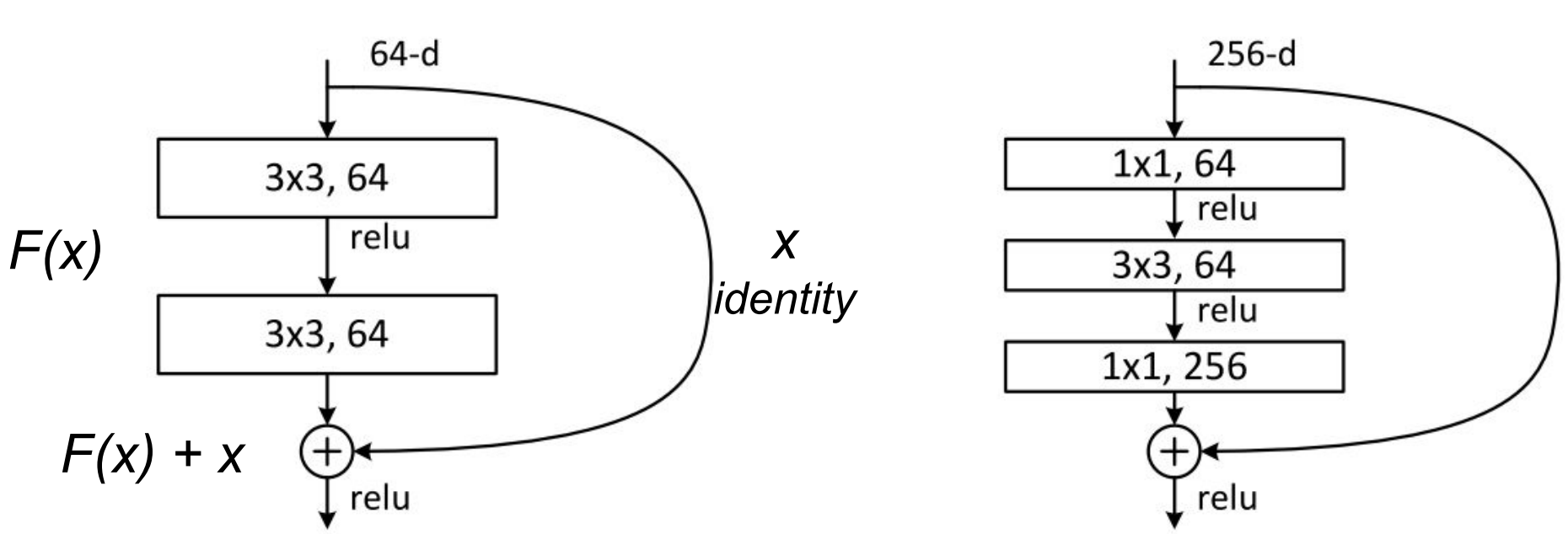
Adapted from: Deep Residual Learning for Image Recognition.

The second, the bottleneck unit, consists of three stacked operations. A series of 1x1, 3x3 and 1x1 convolutions substitute the previous design. The two 1x1 operations are designed for reducing and restoring dimensions. This leaves the 3x3 convolution, in the middle, to operate on a less dense feature vector. Also, BN is applied after each convolution and before ReLU non-linearity.

To help to understand, let’s denote these group of operations as a function F of its input x.

After the non-linear transformations in F(x), the unit combines the result of F(x) with the original input x. This combination is done by adding the two functions. Merging the original input x with the non-linear function F(x) offers some advantages. It allows earlier layers to access the gradient signal from later layers. In other words, skipping the operations on F(x) allows earlier layers to have access to a stronger gradient signal. As a result, this type of connectivity has been shown to ease the training of deeper networks.

Non-bottleneck units also show gain in accuracy as we increase model capacity. Yet, bottleneck residual units have some practical advantages. First, it performs more computations having almost the same number of parameters. Second, they also perform in a similar computational complexity as its counterpart.

In practice, bottleneck units are more suitable for training deeper models because of less training time and computational resources need.

For our implementation, we use the full pre-activation Residual Unit. The only difference, from the standard bottleneck unit, lies in the order in which BN and ReLU activations are placed. For the full pre-activation, BN and ReLU (in this order) occur before convolutions.

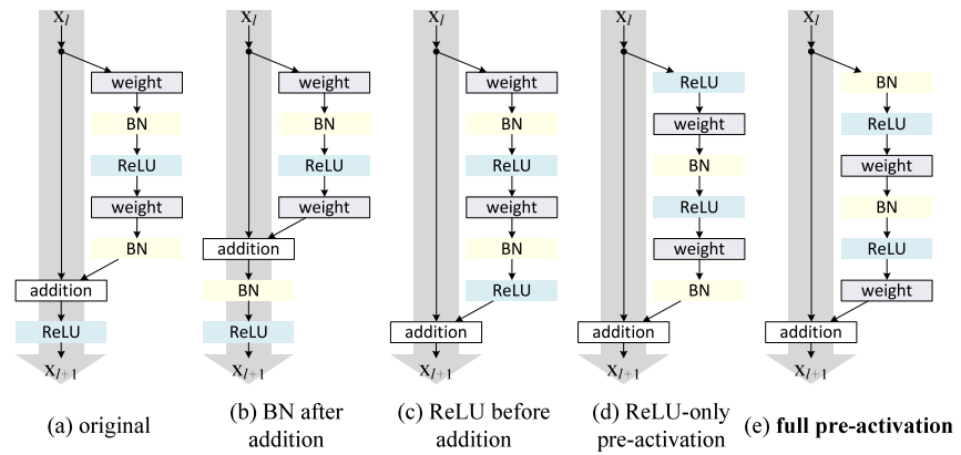
Image credits: Identity Mappings in Deep Residual Networks.

As shown in Identity Mappings in Deep Residual Networks, the full pre-activation unit performs better than other variants.

Note that the only difference between these designs is the order of BN and RELu in the convolution stack.

Atrous Convolutions

Atrous (or dilated) convolutions are regular convolutions with a factor that allows us to expand the filter’s field of view.

Consider a 3x3 convolution filter for instance. When the dilation rate is equal to 1, it behaves like a standard convolution. But, if we set the dilation factor to 2, it has the effect of enlarging the convolution kernel.

In theory, it works like that. First, it expands (dilates) the convolution filter according to the dilation rate. Second, it fills the empty spaces with zeros - creating a sparse like filter. Finally, it performs regular convolution using the dilated filter.

As a consequence, a convolution with a dilated 2, 3x3 filter would make it able to cover an area equivalent to a 5x5. Yet, because it acts like a sparse filter, only the original 3x3 cells will do computation and produce results. I said “act” because most frameworks don’t implement atrous convolutions using sparse filters - because of memory concerns.

In a similar way, setting the atrous factor to 3 allows a regular 3x3 convolution to get signals from a 7x7 corresponding area.

This effect allows us to control the resolution at which we compute feature responses. Also, atrous convolution adds larger context without increasing the number of parameters or the amount of computation.

Deeplab also shows that the dilation rate must be tuned according to the size of the feature maps. They studied the consequences of using large dilation rates over small feature maps.

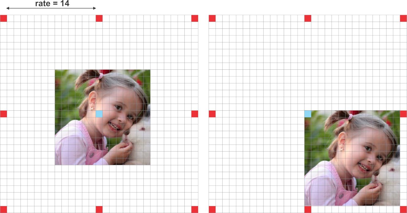
When the dilation rate is very close to the feature map’s size, a regular 3x3 atrous filter acts as a standard 1x1 convolution.

Put in another way, the efficiency of atrous convolutions depends on a good choice of the dilation rate. Because of that, it is important to know the concept of output stride in neural networks.

Output stride explains the ratio of the input image size to the output feature map size. It defines how much signal decimation the input vector suffers as it passes the network.

For an output stride of 16, an image size of 224x224x3 outputs a feature vector with 16 times smaller dimensions. That is 14x14.

Besides, Deeplab also debates the effects of different output strides on segmentation models. It argues that excessive signal decimation is harmful for dense prediction tasks. In short, models with smaller output stride - less signal decimation - tends to output finer segmentation results. Yet, training models with smaller output stride demand more training time.

Deeplab reports experiments with two configurations of output strides, 8 and 16. As expected, output stride = 8 was able to produce slightly better results. Here we choose output stride = 16 for practical reasons.

Also, because the atrous block doesn’t implement downsampling, ASPP also runs on the same feature response size. As a result, it allows learning features from multi-scale context using relative large dilation rates.

The new Atrous Residual Block contains three residual units. In total, the 3 units have three 3x3 convolutions. Motivated by multigrid methods, Deeplab proposes different dilation rates for each convolution. In summary, multigrid defines the dilation rates for each of the three convolutions.

In practice:

For the new block4, when output stride = 16 and Multi Grid = (1, 2, 4), the three convolutions have rates = 2 · (1, 2, 4) = (2, 4, 8) respectively.

Atrous Spatial Pyramid Pooling

For ASPP, the idea is to provide the model with multi-scale information. To do that, ASPP adds a series atrous convolutions with different dilation rates. These rates are designed to capture long-range context. Also, to add global context information, ASPP incorporates image-level features via Global Average Pooling (GAP).

This version of ASPP contains 4 parallel operations. These are a 1x1 convolution and three 3x3 convolutions with dilation rates =(6,12,18). As we mentioned, at this point, the feature maps’ nominal stride is equal to 16.

Based on the original implementation, we use crop sizes of 513x513 for both: training and testing. Thus, using an output stride 16 means that ASPP receives feature vectors of size 32x32.

Also, to add more global context information, ASPP incorporates image-level features. First, it applies GAP to the output features from the last atrous block. Second, the resulting features are fed to a 1x1 convolution with 256 filters. Finally, the result is bilinearly upsampled to the correct dimensions.

@slim.add_arg_scope
def atrous_spatial_pyramid_pooling(net, scope, depth=256):
    """
    ASPP consists of (a) one 1×1 convolution and three 3×3 convolutions with rates = (6, 12, 18) when output stride = 16
    (all with 256 filters and batch normalization), and (b) the image-level features as described in https://arxiv.org/abs/1706.05587
    :param net: tensor of shape [BATCH_SIZE, WIDTH, HEIGHT, DEPTH]
    :param scope: scope name of the aspp layer
    :return: network layer with aspp applyed to it.
    """

    with tf.variable_scope(scope):
        feature_map_size = tf.shape(net)

        # apply global average pooling
        image_level_features = tf.reduce_mean(net, [1, 2], name='image_level_global_pool', keep_dims=True)
        image_level_features = slim.conv2d(image_level_features, depth, [1, 1], scope="image_level_conv_1x1", activation_fn=None)
        image_level_features = tf.image.resize_bilinear(image_level_features, (feature_map_size[1], feature_map_size[2]))

        at_pool1x1 = slim.conv2d(net, depth, [1, 1], scope="conv_1x1_0", activation_fn=None)

        at_pool3x3_1 = slim.conv2d(net, depth, [3, 3], scope="conv_3x3_1", rate=6, activation_fn=None)

        at_pool3x3_2 = slim.conv2d(net, depth, [3, 3], scope="conv_3x3_2", rate=12, activation_fn=None)

        at_pool3x3_3 = slim.conv2d(net, depth, [3, 3], scope="conv_3x3_3", rate=18, activation_fn=None)

        net = tf.concat((image_level_features, at_pool1x1, at_pool3x3_1, at_pool3x3_2, at_pool3x3_3), axis=3,
                        name="concat")
        net = slim.conv2d(net, depth, [1, 1], scope="conv_1x1_output", activation_fn=None)
        return net

In the end, the features, from all the branches, are combined into a single vector via concatenation. This output is then convoluted with another 1x1 kernel - using BN and 256 filters.

After ASPP, we feed the result to another 1x1 convolution - to produce the final segmentation logits.

Implementation Details

Using the ResNet-50 as feature extractor, this implementation of Deeplab_v3 employs the following network configuration:

• output stride = 16
• Fixed multi-grid atrous convolution rates of (1,2,4) to the new Atrous Residual block (block 4).
• ASPP with rates (6,12,18) after the last Atrous Residual block.

Setting output stride to 16 gives us the advantage of substantially faster training. Comparing to output stride of 8, stride of 16 makes the Atrous Residual block deals with 4 times smaller feature maps than its counterpart.

The multi-grid dilation rates are applied to the 3 convolutions inside the Atrous Residual block.

Finally, each of the three parallel 3x3 convolutions in ASPP gets a different dilation rate - (6,12,18).

Before computing the cross-entropy error, we resize the logits to the input’s size. As argued in the paper, it’s better to resize the logits than the ground-truth labels to keep resolution details.

Based on the original training procedures, we scale each image using a random factor from 0.5 to 2. Also, we apply random left-right flipping to the scaled images.

Finally, we crop patches of size 513x513 for both training and testing.

def deeplab_v3(inputs, args, is_training, reuse):

    # mean subtraction normalization
    inputs = inputs - [_R_MEAN, _G_MEAN, _B_MEAN]

    # inputs has shape [batch, 513, 513, 3]
    with slim.arg_scope(resnet_utils.resnet_arg_scope(args.l2_regularizer, is_training,
                                                      args.batch_norm_decay,
                                                      args.batch_norm_epsilon)):
        resnet = getattr(resnet_v2, args.resnet_model) # get one of the resnet models: resnet_v2_50, resnet_v2_101 ...
        _, end_points = resnet(inputs,
                               args.number_of_classes,
                               is_training=is_training,
                               global_pool=False,
                               spatial_squeeze=False,
                               output_stride=args.output_stride,
                               reuse=reuse)

        with tf.variable_scope("DeepLab_v3", reuse=reuse):

            # get block 4 feature outputs
            net = end_points[args.resnet_model + '/block4']

            net = atrous_spatial_pyramid_pooling(net, "ASPP_layer", depth=256, reuse=reuse)

            net = slim.conv2d(net, args.number_of_classes, [1, 1], activation_fn=None,
                              normalizer_fn=None, scope='logits')

            size = tf.shape(inputs)[1:3]
            # resize the output logits to match the labels dimensions
            #net = tf.image.resize_nearest_neighbor(net, size)
            net = tf.image.resize_bilinear(net, size)
            return net

To implement atrous convolutions with multi-grid in the block4 of the resnet, we just changed this piece in the resnet_utils.py file.

...
with tf.variable_scope('unit_%d' % (i + 1), values=[net]):
  # If we have reached the target output_stride, then we need to employ
  # atrous convolution with stride=1 and multiply the atrous rate by the
  # current unit's stride for use in subsequent layers.
  if output_stride is not None and current_stride == output_stride:
    # Only uses atrous convolutions with multi-graid rates in the last (block4) block
    if block.scope == "block4":
      net = block.unit_fn(net, rate=rate * multi_grid[i], **dict(unit, stride=1))
    else:
      net = block.unit_fn(net, rate=rate, **dict(unit, stride=1))
    rate *= unit.get('stride', 1)
...

Training

To train the network, we decided to use the augmented Pascal VOC dataset provided by Semantic contours from inverse detectors.

The training data is composed of 8,252 images. 5,623 from the training set and 2,299 from the validation set. To test the model using the original VOC 2012 val dataset, I removed 558 images from the 2,299 validation set. These 558 samples were also present on the official VOC validation set. Also, I added 330 images from the VOC 2012 train set that weren’t present either among the 5,623 nor the 2,299 sets. Finally, 10% of the 8,252 images (~825 samples) are held for validation, leaving the rest for training.

Note that different from the original paper, this implementation is not pre-trained in the COCO dataset. Also, some of the techniques described in the paper for training and evaluation were not queried out.

Results

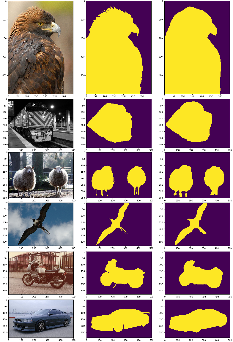
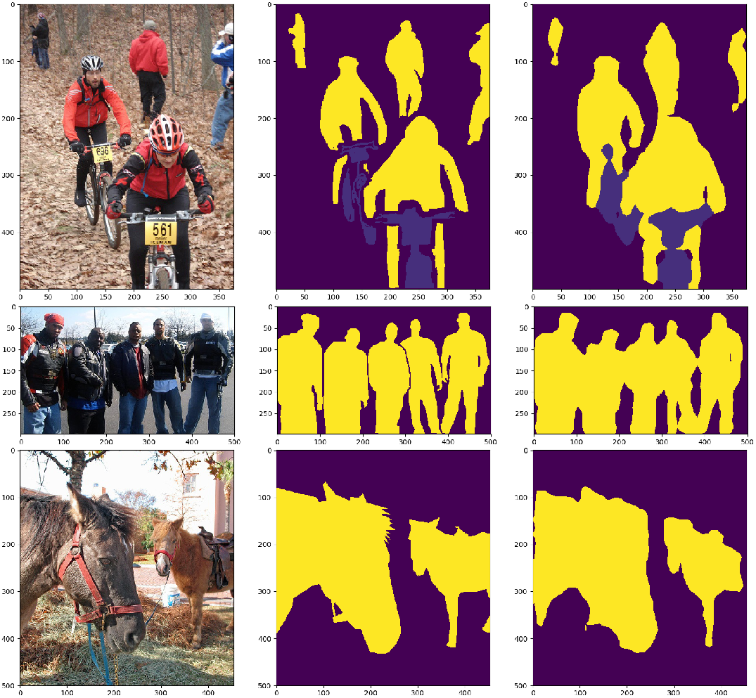
The model was able to achieve decent results on the PASCAL VOC validation set.

• Pixel accuracy: ~91%
• Mean Accuracy: ~82%
• Mean Intersection over Union (mIoU): ~74%
• Frequency weighed Intersection over Union: ~86%.

Bellow, you can check out some of the results in a variety of images from the PASCAL VOC validation set.

Concluding

The field of Semantic Segmentation is no doubt one of the hottest ones in Computer Vision. Deeplab presents an alternative to classic encoder-decoder architectures. It advocates the usage of atrous convolutions for feature learning in multi-range contexts. Feel free to clone the repo and tune the model to achieve closer results to the original implementation. The complete code is here.

Hope you like reading!

Cite as:

@article{
  silva2018semanticsegmentation,
  title={Deeplab Image Semantic Segmentation Network},
  author={Silva, Thalles Santos},
  journal={https://sthalles.github.io},
  year={2018}
  url={https://sthalles.github.io/deep_segmentation_network/}
}