Densely Connected Convolutional Networks in Tensorflow
[machine-learning deep-learning representation-learning classification densenets tensorflow 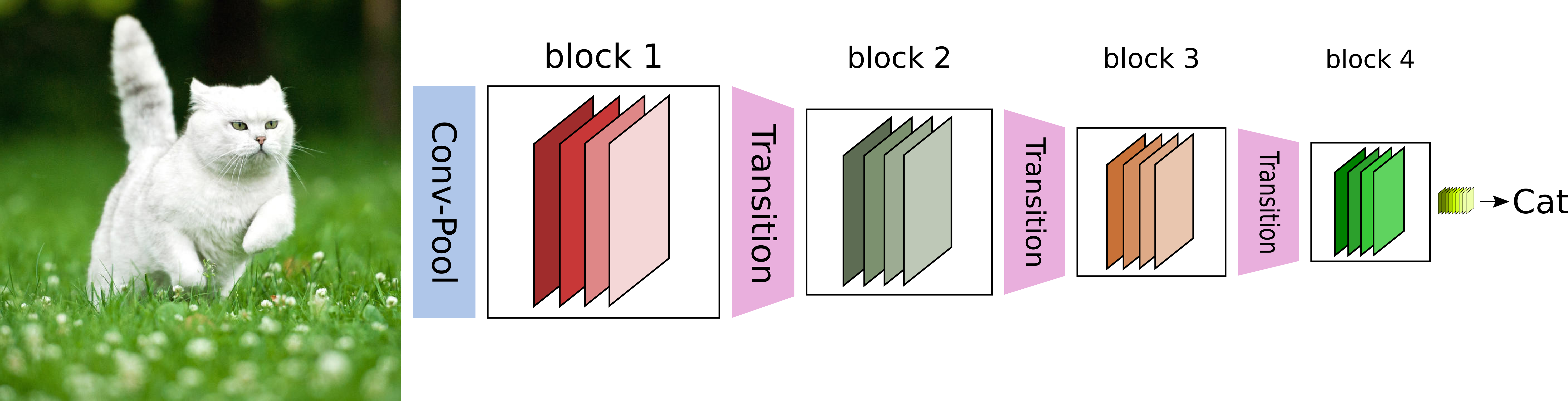
Intro
If you like Neural Nets, you certainly have heard about the VGGNet, Resnet, Inception, and others. These networks, each one in its time, reached state-of-the-art performance in some of the most famous challenges in Computer Vision. If we look at the short and successful history of Deep Neural Networks, we see an interesting trend. Mainly, after the the GPGPU and big data revolutions, we notice that year by year, these models got deeper and more powerful. However, as networks were getting denser in the number of parameters and layers, the problem of how to prevent the gradient from vanishing, by the time it reaches the first layers of the model, was something to worry about.
To address this issue, many network architectures such as Resnets and Highway networks emerged. Besides some changes, all of them tried to solve this problem using a very similar approach. To create shortcut connections that bypass a group of operations so that the gradient signal could be propagated without much loss from the end to the beginning of the network.
In this context, arouse the Densely Connected Convolutional Networks, DenseNets.
I have been using this architecture for a while in at least two different kinds of problems, classification and densely prediction tasks such as semantic segmentation. During this time, I developed a Library to use DenseNets using Tensorflow with its Slim package. In this post, we are going to do an overview of the DenseNet architecture. We compare it with other very popular models, and show how one might use the Library for its own pleasure.
Network Architecture
To understand DenseNets, we need to focus on two principal components of its architecture. The Dense Block, and the Transition Layer.
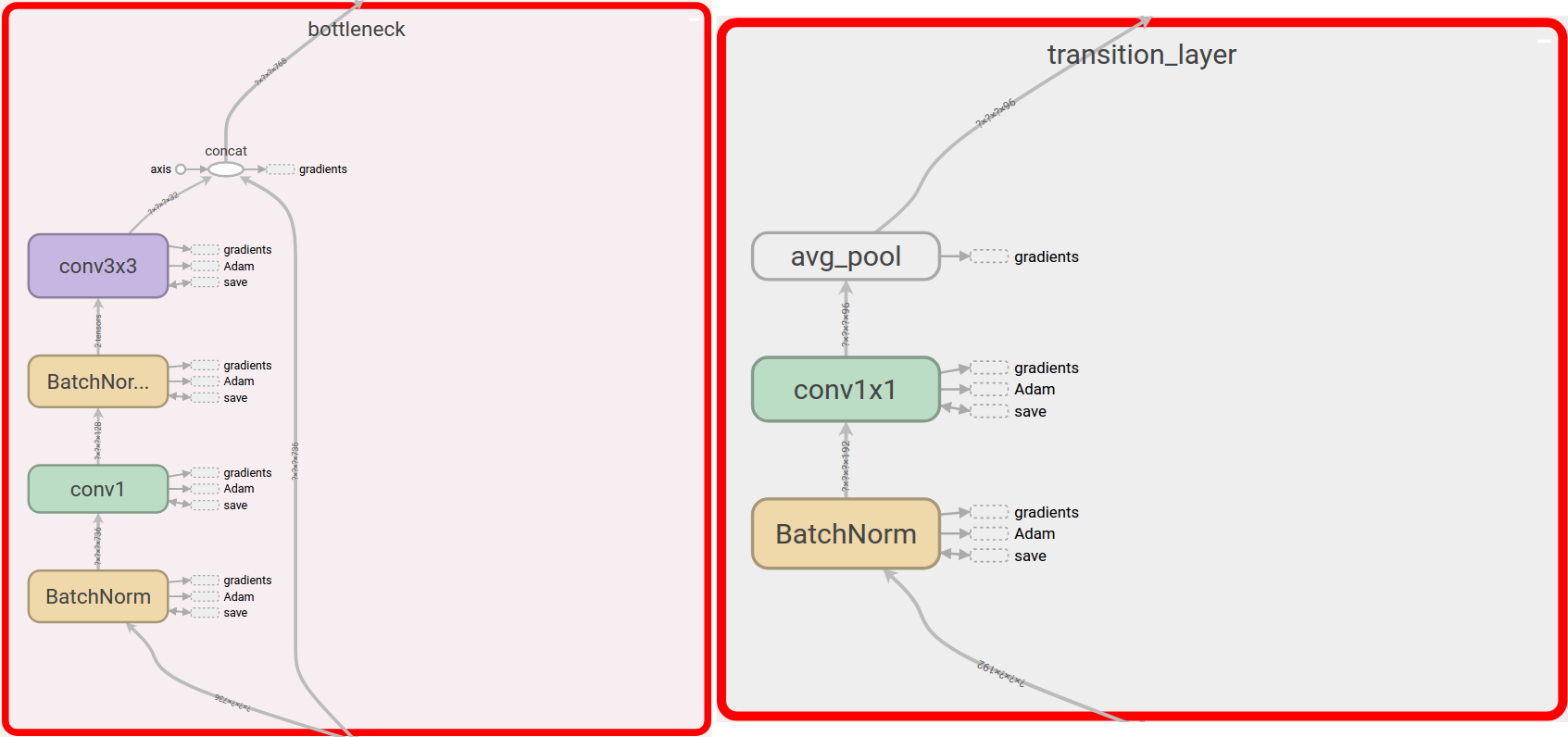
A DenseNet is a stack of dense blocks followed by transition layers. Each block consists of a series of units. Each unit packs two convolutions, each preceded by Batch Normalization and ReLU activations. Besides, each unit outputs a fixed number of feature vectors. This parameter, described as the growth rate, controls how much new information the layers allow to pass through.
On the other hand, transition layers are very simple components designed to perform downsampling of the features passing the network. Every transition layer consists of a Batch Normalization layer, followed by a 1x1 convolution, followed by a 2x2 average pooling.
The big difference from other regular CNNs, is that each unit within a dense block is connected to every other unit before it. In summary, within a given block, the nth unit, receives as input the feature-maps learned by the n-1, n-2, … all the way down to the 1st unit in the pipeline. As a result, it allows DenseNets to carry very few parameters because there is a very high level of feature sharing amongst the units. We will talk more about number of parameters in a bit.
Different from ResNets, DenseNets propose feature reuse among units by concatenation. As a consequence of that choice, DenseNets tend to be more compact (in the number of parameters) than ResNets. Intuitively, every feature-map learned by any given DenseNet unit is reused by all of the following units within a block. As a result, it minimizes the possibility of different layers of the network to learn redundant features.
To get a better glance at it, let’s have a look at the differences between a ResNet unit and a DenseNet unit. Both architectures use the so called bottleneck layer. This design usually contains a 1x1 convolution to reduce features’ spatial dimensions, followed by a wider convolution, in this case a 3x3 operation for feature learning.
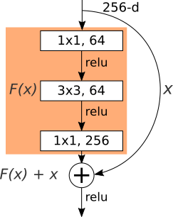
In its original form, the ResNet bottleneck layer consists of a 1x1 followed by a 3x3 followed by another 1x1 convolution, closing with an addition operation between the original input and the result of the non-linear transformations. This connection between the non-linear transformations f(x) and the original input x, provides a way to make the gradient signal from the later layers (where it is probably stronger) to be sent directly to earlier layers, skipping the operations on f(x) - where the gradient might be diminished.
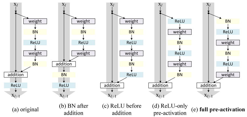
This very elegant design gave the ResNet the ILSVRC 2015 classification task challenge championship and since then, it inspired many others similar architectures that improved upon it, as shown in Figure 3 - credits: Identity Mappings in Deep Residual Networks .
Regarding parameter efficiency and floating point operations per second (FLOPs), DenseNets not only achieve smaller error rates (on ImageNet) but they also need less parameters and less float point operations than ResNets.
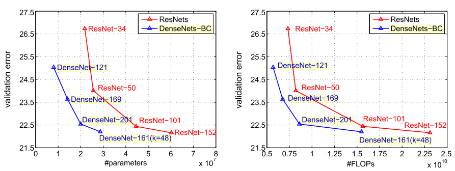
Another trick that enhances model compactness is the feature-map filtering operation carry out on the DenseNets’ transition layers. To reduce the number of feature vectors that go into each dense block, DenseNets implement a filtering mechanism where in each transition layer, a factor θ, between 0 and 1, controls how much of the current features are allowed to pass through to the following block. In this context, DenseNets that implement the bottleneck layer described above and a value of θ < 1 are called DenseNets-BC and are the most parameter efficient variation.
Library
The DenseNet Library is heavily based on the resnet_v2 library available on the Tensorflow Slim package. That follows a basic usage for classification task with 1000 classes.
import tensorflow as tf
import numpy as np
import densenet
from densenet_utils import densenet_arg_scope
slim = tf.contrib.slim

fake_input = np.zeros((1,224,224,3), dtype=np.float32)

with slim.arg_scope(densenet_arg_scope()):
    net, end_points = densenet.densenet_121(inputs=fake_input,
                                            num_classes=1000,
                                            theta=0.5,
                                            is_training=True,
                                            scope='DenseNet_121')
    print(net.shape)# (1, 1000)
By default, DenseNets have nominal stride equal to 32, that is, the ratio of the input image resolution to the final output resolution is 32. An output stride of 32 means that after four DenseNet blocks and respective transition layers, an input image with size (BATCH_SIZE, 224, 224, 3) will be down sampled to a tensor of shape (BATCH_SIZE, 7, 7, DEPTH).
Finally, to output the final result, a global average pooling followed by a fully connected op is applied to output a vector with shape (BATCH_SIZE, num_classes).
However, for dense prediction tasks such as semantic segmentation, one might benefit setting the output stride to something smaller such as 16 or even 8. Now, follows the example where we use output_stride=16, deactivate global average pooling and note the initial_output_stride parameter set to 2.
with slim.arg_scope(densenet_arg_scope()):

    net, end_points = densenet.densenet_121(fake_input,
                                   num_classes=21,
                                   theta=0.5,
                                   is_training=True,
                                   global_pool=False,
                                   output_stride=16,
                                   initial_output_stride=2,
                                   spatial_squeeze=False)
    with tf.Session() as sess:
      sess.run(tf.global_variables_initializer())
      logits = sess.run(net)
      print(logits.shape) # (1, 14, 14, 21)
Different than the first setup, now we get a tensor shape of (BATCH_SIZE, 14, 14, 21) suitable for segmentation like problems. The initial_output_stride input argument was conceived to control how much of signal decimation one desires before the dense blocks.
In the original DenseNet paper, right before the first dense block, a strided 2 convolution and a max pooling operations are performed to reduce spatial information even further. That original choice is designed for processing large batches of images and still be able to load them on GPU. However, for semantic segmentation problems, or if one uses relative small inputs like CIFAR-10 like images with size 64x64, it might be worth to control that downsampling rate.
When setting initial_output_stride to 2, the network will only convolve the input image to 2 * growth_rate filters and skip the max pooling operation.
The Library offers all 4 architecture implementations used to train on ImageNet. For densenet_121(…), densenet_169(…), densenet_201(…) the growth_rate is set to 32 while for densenet_161(…), the value growth_rate is set to 48 as described in the paper.
with slim.arg_scope(densenet_arg_scope()):

    net, end_points = densenet.densenet_121(...)
    net, end_points = densenet.densenet_169(...)
    net, end_points = densenet.densenet_201(...)
    net, end_points = densenet.densenet_161(...)
However, if one feels like playing with different setups, there is the densenet.densenet_X(…) constructor, where the number of dense blocks, the number of units within each block as well as the growth_rate factor can be manually configured.
# Custom definition for DenseNet_121
def densenet_X(inputs,
                num_classes=None,
                theta=0.5,
                num_units_per_block=[6,12,24,16], # number of blocks equal to 4
                growth_rate=32,
                is_training=True,
                global_pool=True,
                output_stride=None,
                spatial_squeeze=True,
                initial_output_stride=4,
                reuse=None,
                scope='DenseNet_X'):
Concluding
DenseNets offer very scalable models that achieve very good accuracy and are easy to train. The key idea consists sharing feature maps within a block through direct connections between layers. Moreover, it demands fewer parameters than a number of other models like ResNets, Inception Networks, and others while offering equally or improved accuracy on various classification datasets. The DenseNet library described here implements all 4 architectures used to train on ImageNet plus a custom constructor in which any network variation can be experimented. Feel free to checkout the code on Github and make pull requests with any suggestion.
Cite as:
@article{
  silva2017densenets,
  title={Densely Connected Convolutional Networks in Tensorflow},
  author={Silva, Thalles Santos},
  journal={https://sthalles.github.io},
  year={2017}
  url={https://sthalles.github.io/densely-connected-conv-nets/}
}