An illustrative introduction to Fisher's Linear Discriminant
[machine-learning deep-learning dimensionality-reduction pca representation-learning 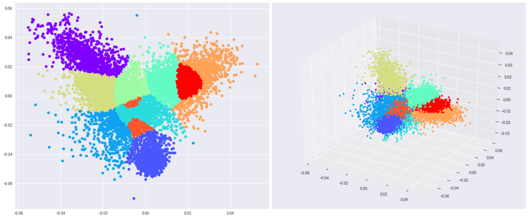
Introduction
To deal with classification problems with 2 or more classes, most Machine Learning (ML) algorithms work the same way.
Usually, they apply some kind of transformation to the input data with the effect of reducing the original input dimensions to a new (smaller) one. The goal is to project the data to a new space. Then, once projected, they try to classify the data points by finding a linear separation.
For problems with small input dimensions, the task is somewhat easier. Take the following dataset as an example.
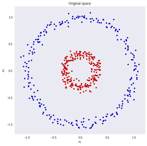
Suppose we want to classify the red and blue circles correctly. It is clear that with a simple linear model we will not get a good result. There is no linear combination of the inputs and weights that maps the inputs to their correct classes. But what if we could transform the data so that we could draw a line that separates the 2 classes?
That is what happens if we square the two input feature-vectors. Now, a linear model will easily classify the blue and red points.
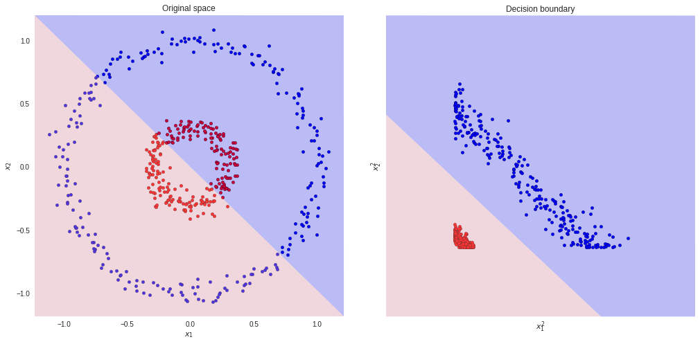
However, sometimes we do not know which kind of transformation we should use. Actually, to find the best representation is not a trivial problem. There are many transformations we could apply to our data. Likewise, each one of them could result in a different classifier (in terms of performance).
One solution to this problem is to learn the right transformation. This is known as representation learning and it is exactly what you are thinking - Deep Learning. The magic is that we do not need to “guess” what kind of transformation would result in the best representation of the data. The algorithm will figure it out.
However, keep in mind that regardless of representation learning or hand-crafted features, the pattern is the same. We need to change the data somehow so that it can be easily separable.
Let’s take some steps back and consider a simpler problem.
In this piece, we are going to explore how Fisher’s Linear Discriminant (FLD) manages to classify multi-dimensional data. But before we begin, feel free to open this Colab notebook and follow along.
Fisher’s Linear Discriminant
We can view linear classification models in terms of dimensionality reduction.
To begin, consider the case of a two-class classification problem (K=2). Blue and red points in R². In general, we can take any D-dimensional input vector and project it down to D’-dimensions. Here, D represents the original input dimensions while D’ is the projected space dimensions. Throughout this article, consider D’ less than D.
In the case of projecting to one dimension (the number line), i.e. D’=1, we can pick a threshold t to separate the classes in the new space. Given an input vector x:
- if the predicted value y >= t then, x belongs to class C1 (class 1) - where
.
- otherwise, it is classified as C2 (class 2).
Take the dataset below as a toy example. We want to reduce the original data dimensions from D=2 to D’=1. In other words, we want a transformation T that maps vectors in 2D to 1D - T(v) = ℝ² →ℝ¹.
First, let’s compute the mean vectors m1 and m2 for the two classes.
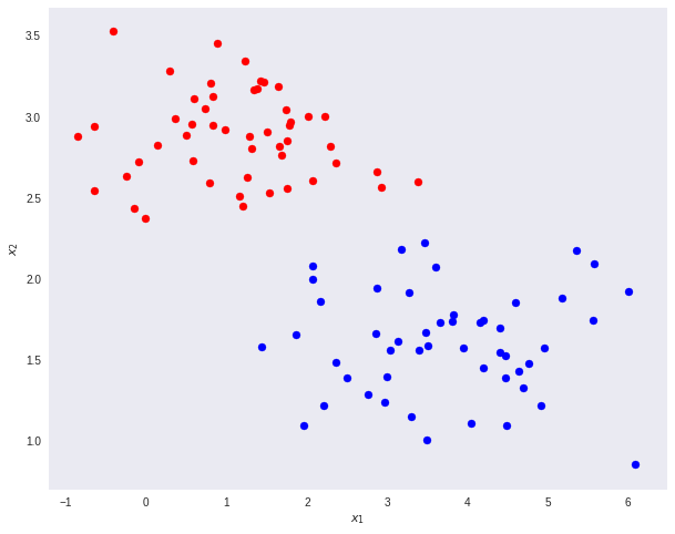

Note that N1 and N2 denote the number of points in classes C1 and C2 respectively. Now, consider using the class means as a measure of separation. In other words, we want to project the data onto the vector W joining the 2 class means.
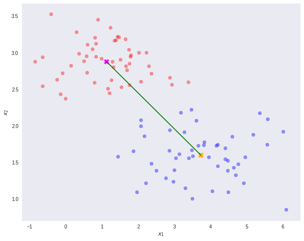
It is important to note that any kind of projection to a smaller dimension might involve some loss of information. In this scenario, note that the two classes are clearly separable (by a line) in their original space.
However, after re-projection, the data exhibit some sort of class overlapping - shown by the yellow ellipse on the plot and the histogram below.
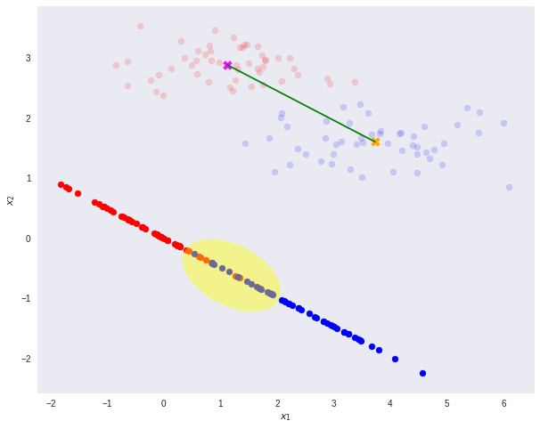
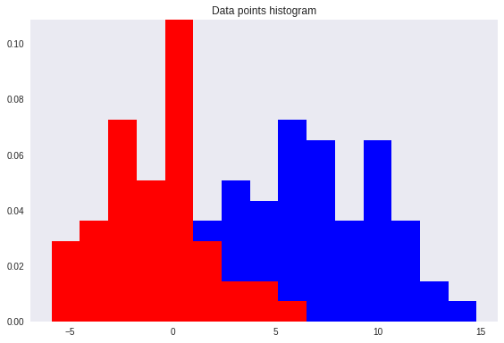
That is where the Fisher’s Linear Discriminant comes into play.
The idea proposed by Fisher is to maximize a function that will give a large separation between the projected class means while also giving a small variance within each class, thereby minimizing the class overlap.
In other words, FLD selects a projection that maximizes the class separation. To do that, it maximizes the ratio between the between-class variance to the within-class variance.
In short, to project the data to a smaller dimension and to avoid class overlapping, FLD maintains 2 properties.
- A large variance among the dataset classes.
- A small variance within each of the dataset classes.
Note that a large between-class variance means that the projected class averages should be as far apart as possible. On the contrary, a small within-class variance has the effect of keeping the projected data points closer to one another.

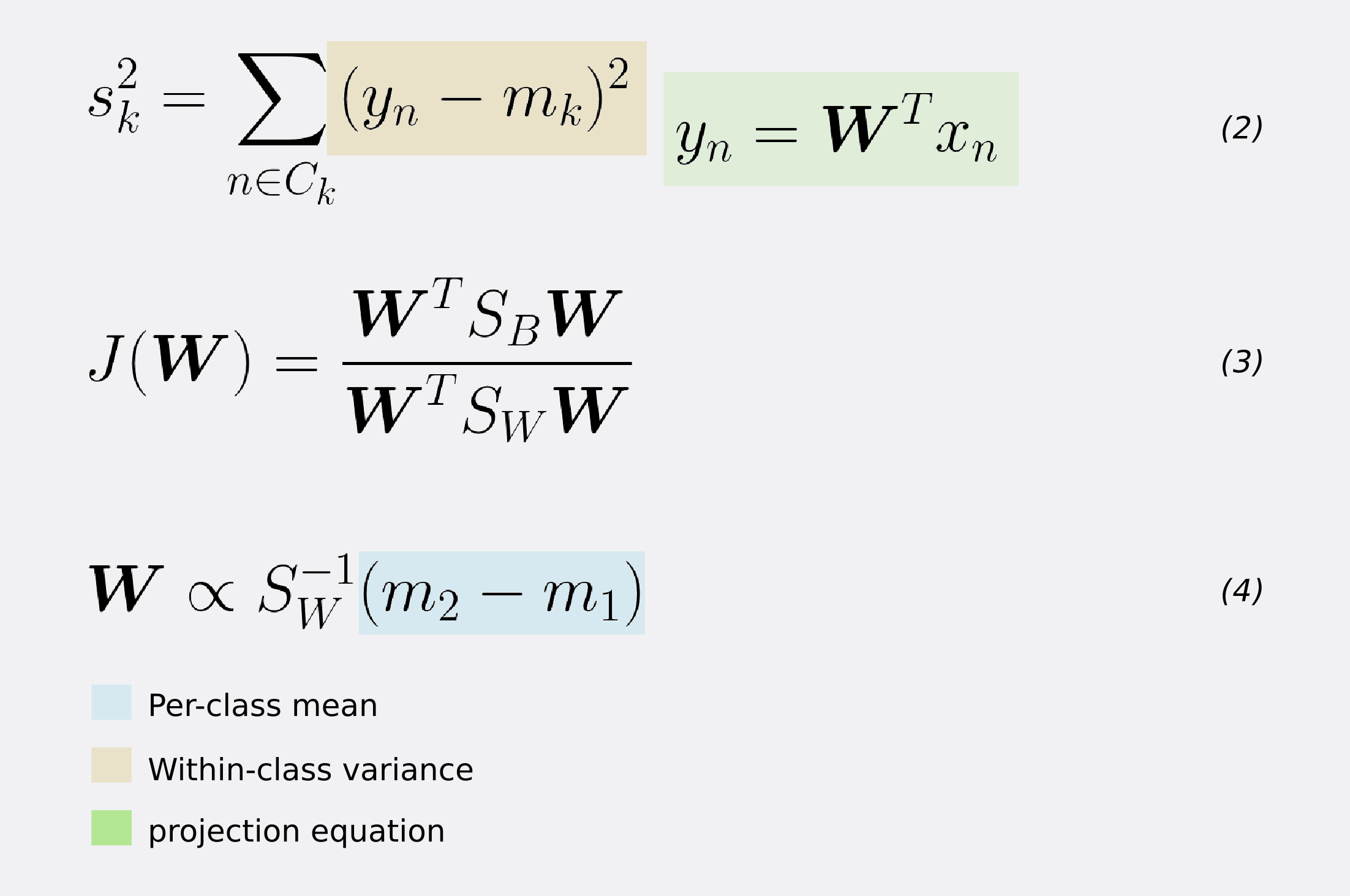
To find the projection with the following properties, FLD learns a weight vector W with the following criterion.
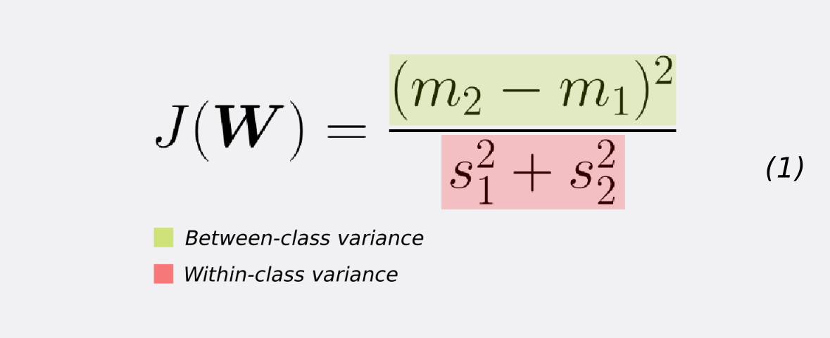
If we substitute the mean vectors m1 and m2 as well as the variance s as given by equations (1) and (2) we arrive at equation (3). If we take the derivative of (3) w.r.t W (after some simplifications) we get the learning equation for W (equation 4). That is, W (our desired transformation) is directly proportional to the inverse of the within-class covariance matrix times the difference of the class means.
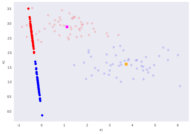
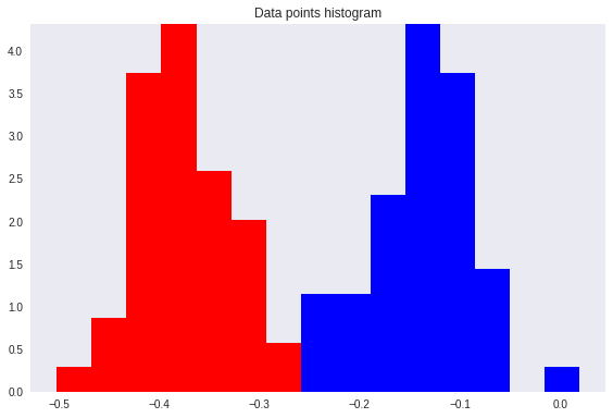
As expected, the result allows a perfect class separation with simple thresholding.
Fisher’s Linear Discriminant for Multiple Classes
We can generalize FLD for the case of more than K>2 classes. Here, we need generalization forms for the within-class and between-class covariance matrices.
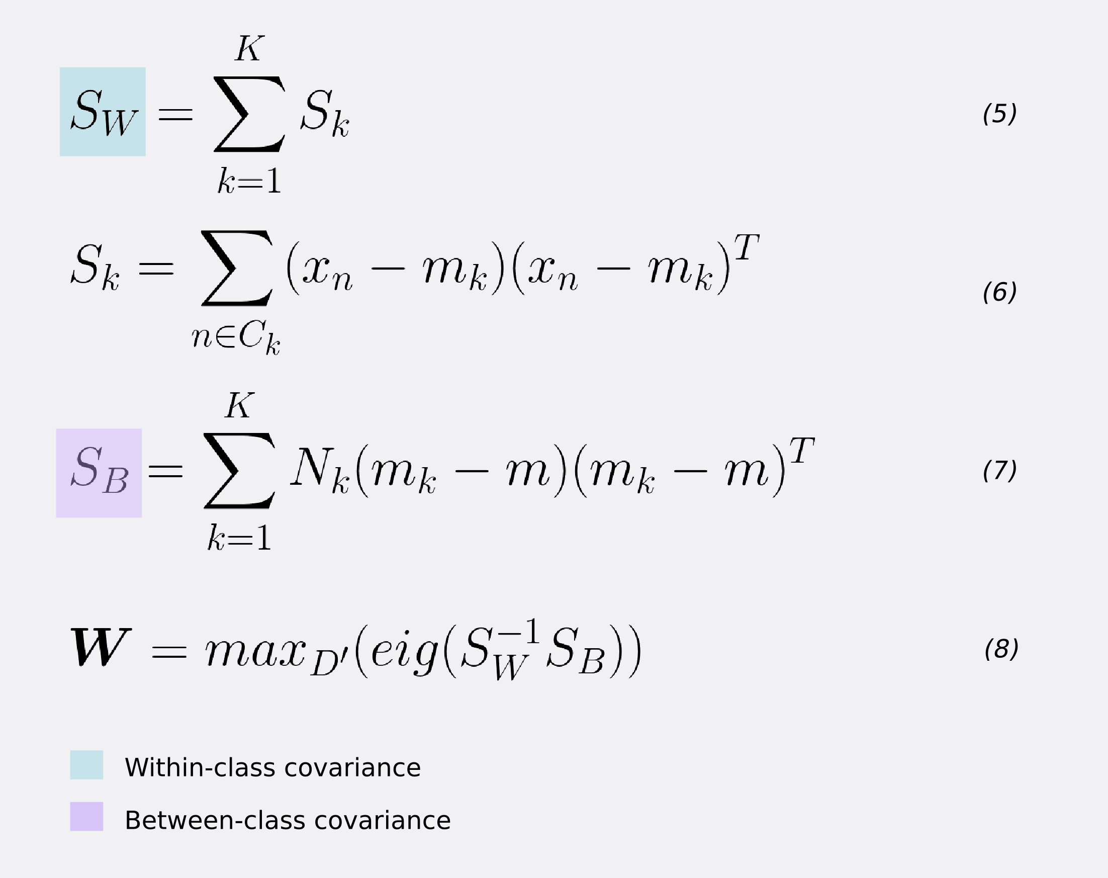
For the within-class covariance matrix SW, for each class, take the sum of the matrix-multiplication between the centralized input values and their transpose. Equations 5 and 6.
For estimating the between-class covariance SB, for each class k=1,2,3,…,K, take the outer product of the local class mean mk and global mean m. Then, scale it by the number of records in class k - equation 7.
The maximization of the FLD criterion is solved via an eigendecomposition of the matrix-multiplication between the inverse of SW and SB. Thus, to find the weight vector **W**, we take the **D’** eigenvectors that correspond to their largest eigenvalues (equation 8).
In other words, if we want to reduce our input dimension from D=784 to D’=2, the weight vector W is composed of the 2 eigenvectors that correspond to the D’=2 largest eigenvalues. This gives a final shape of W = (N,D’), where N is the number of input records and D’ the reduced feature dimensions.
Building a linear discriminant
Up until this point, we used Fisher’s Linear discriminant only as a method for dimensionality reduction. To really create a discriminant, we can model a multivariate Gaussian distribution over a D-dimensional input vector x for each class K as:

Here μ (the mean) is a D-dimensional vector. Σ (sigma) is a DxD matrix - the covariance matrix. And |Σ| is the determinant of the covariance. In python, it looks like this.
The parameters of the Gaussian distribution: μ and Σ, are computed for each class k=1,2,3,…,K using the projected input data. We can infer the priors P(Ck) class probabilities using the fractions of the training set data points in each of the classes (line 11).
Once we have the Gaussian parameters and priors, we can compute class-conditional densities P(x|Ck) for each class k=1,2,3,…,K individually. To do it, we first project the D-dimensional input vector x to a new D’ space. Keep in mind that D < D’. Then, we evaluate equation 9 for each projected point. Finally, we can get the posterior class probabilities P(Ck|x) for each class k=1,2,3,…,K using equation 10.

Equation 10 is evaluated on line 8 of the score function below.
We then can assign the input vector x to the class k ∈ K with the largest posterior.
Testing on MNIST
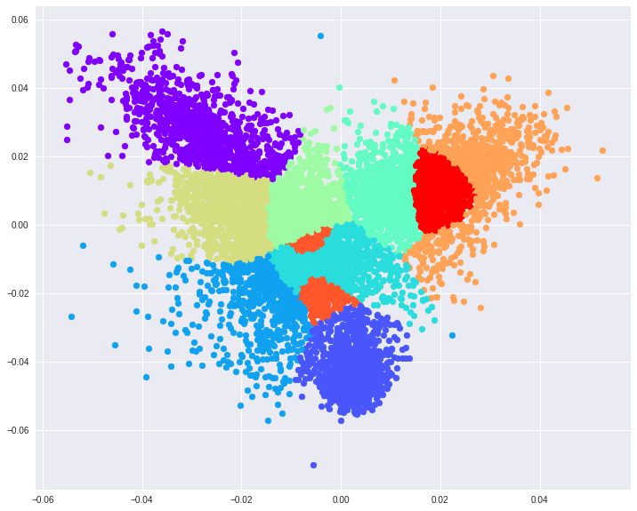
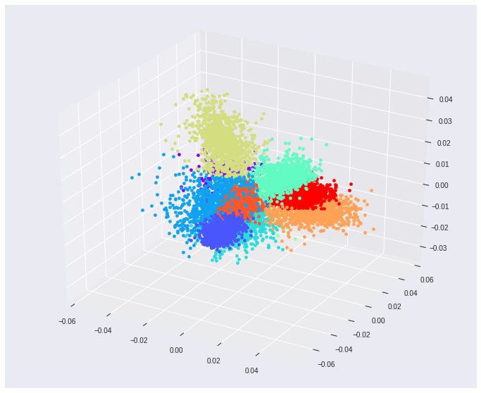
Using MNIST as a toy testing dataset. If we choose to reduce the original input dimensions D=784 to D’=2 we get around 56% accuracy on the test data. If we increase the projected space dimensions to D’=3, however, we reach nearly 74% accuracy. These 2 projections also make it easier to visualize the feature space.
Some key takeaways from this piece.
-
Fisher’s Linear Discriminant, in essence, is a technique for dimensionality reduction, not a discriminant. For binary classification, we can find an optimal threshold t and classify the data accordingly. For multiclass data, we can (1) model a class conditional distribution using a Gaussian. (2) Find the prior class probabilities P(Ck), and (3) use Bayes to find the posterior class probabilities
p(Ck|x). -
To find the optimal direction to project the input data, Fisher needs supervised data.
-
Given a dataset with D dimensions, we can project it down to at most D’ equals to D-1 dimensions.
This article is based on chapter 4.1.6 of Pattern Recognition and Machine Learning. Book by Christopher Bishop
Thanks for reading!
Cite as:
@article{
  silva2019fisherdiscriminant,
  title={An illustrative introduction to Fisher's Linear Discriminant},
  author={Silva, Thalles Santos},
  journal={https://sthalles.github.io},
  year={2019}
  url={https://sthalles.github.io/fisher-linear-discriminant/}
}