Logistic Regression: The good parts

Introduction

In the last post, we tackled the problem of Machine Learning classification through the lens of dimensionality reduction. We saw how Fisher’s Linear Discriminant can project data points from higher to smaller dimensions. The projection follows two principles.

It maximizes the between-class variance.
It minimizes the within-class variance.

Even though Fisher’s method is not (in essence) a discriminant, we built one by modeling a class conditional distribution using a Gaussian. First, we found the prior class probabilities p(Ck). Then, we used Bayes theorem to find the posterior class probabilities p(Ck|x). Here, x is the input vector and Ck is the label for class k.

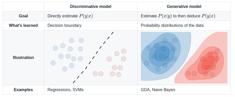
In short, we can categorize ML models based on the way they classify data. There are two types: generative and discriminative methods.

Generative methods learn the posterior class probabilities explicitly. As opposed to it, discriminative algorithms learn the posterior class probabilities directly.

Intuitively, it has a nice geometrical interpretation. For each class, generative models are concerned to find a probabilistic representation of the data. On the contrary, discriminative algorithms focus on separating the data by decision boundaries.

In other words, generative models try to explain the data by building a statistical model for each class.

On the other hand, the goal of a discriminative algorithm is to find an optimal decision boundary that separates the classes. Thus, as long as there is a decision surface, such models do not care about the distributions of the data.

Take a binary classification problem as an example. Given an input vector x, we need to decide to which class Ck, x is most likely to belong to. To make this decision, both types of ML algorithms need a way to compute the posterior probability p(Ck|x) from the training data.

For Fisher’s, we explicitly learned posterior class probabilities using a Gaussian. Once we found it, we used decision theory to determine class membership for x.

For a discriminative model, the posterior p(Ck|x) will be directly derived. In this case, once we have the posterior, we can use decision theory and assign x to the most probable class.

Logistic Regression

Before we begin, make sure you follow along with these Colab notebooks.

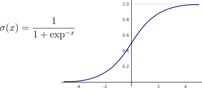
Logistic Regression is probably the best known discriminative model. As such, it derives the posterior class probability p(Ck|x) implicitly.

For binary classification, the posterior probabilities are given by the sigmoid function σ applied over a linear combination of the inputs ϕ.

Similarly, for multiclass problems, we can estimate the posterior using the softmax function. Like the sigmoid, softmax normalizes a given vector to probabilities — values between 0 and 1.

Let’s begin with the case of binary classification.

Binary Logistic Regression

For an M-dimensional input feature-vector, Logistic Regression has to learn M parameters.

Take the SVHN dataset as an example. Each RGB image has a shape of 32x32x3. Thus, logistic regression needs to learn 32x32x3=3072 parameters.

To find the optimal weight values, we usually optimize the cross-entropy error function.

The cross-entropy, or the negative logarithm of the likelihood, measures how far the model’s predictions are from the labels. It increases when the predicted values deviate from the targets and decrease otherwise.

Assuming target values t to be either 0 or 1, cross-entropy is defined as:

Here, N denotes the total number of instances in the dataset and yᵢ are the model’s probabilities.

Cross-entropy compares 2 probability distributions. Because of that, it is important to note that the output of logistic regression is interpreted as probabilities — even during learning.

Taking the derivative of the cross-entropy with respect to the weight vector w, we get the gradient.

Note that to compute this derivative, we need the derivative of the sigmoid function w.r.t weights w.

Luckily, one nice property of the sigmoid is that we can express its derivative in terms of itself.

The gradient is a vector-valued function. In fact, the gradient is a linear transformation that maps input vectors to other vectors of the same shape.

The gradient captures the derivative of a whole multi-variable function. Each one of its values denotes the direction in which we can change one specific weight so that we can reach the maximum point of a function. Thus, the gradient represents the direction of steepest ascent.

Softmax Regression

For multiclass classification, only a few things change. Now, we can model the posterior probabilities using a softmax function.

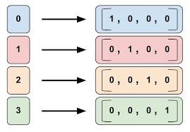
Since logistic regression treats its predictions as probabilities, we need to change the way we represent our labels.

Up to this point, the target/label vector is represented as a vector of integers. In this vector, each value represent a different class. If we want them to be equally valued probabilities, they need to be between 0 and 1. To do this, we can change their representation to one-hot-encodings.

This time, for inputs with M features and K different classes, logistic regression learns MxK parameters. We can view it as the following matrix.

Now, we can proceed similarly to the case of binary classification. First, we take the derivative of the softmax with respect to the activations. Then, the negative logarithm of the likelihood gives us the cross-entropy function for multi-class classification.

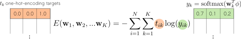
In practice, cross-entropy measures the distance between two vectors of probabilities. One, that comes out of the softmax. And a second containing the one-hot-encoding representations of the true target values.

Note the difference between the error functions used for binary and multiclass classification. In reality, they are really the same thing.

The binary cross-entropy treats the targets as scalars. They take either 0 or 1. For multiclass problems, targets are represented as one-hot-encoded vectors.

Finally, we take the gradient of the error function w.r.t the weights w and obtain the following gradient vectors.

Iterative Reweighted Least Squares

Different from linear regression, logistic regression does not have a closed form solution. In other words, for linear regression, we can solve for a point of gradient equal 0 with the following equation:

For logistic regression, such a closed-form equation does not exist. Thanks to the nonlinearity we apply on the linear combination of the inputs.

However, the relationship between the loss function and the parameters w still gives us a concave error function. Thus, we can rest assured that there is only a unique minimum on the error surface.

As a result, we can solve for it using an iterative technique such as gradient descent or Newton-Raphson.

If we choose gradient descent, we have everything set.

Just follow the opposite direction of the gradient.

In plain English, the direction of steepest descent. As such, we can iteratively update the weightsw as:

Note the minus sign there. It represents the fact that we are going downhill as opposed to uphill.*

However, we can do a little better.

Gradient descent offers the direction of steepest descent to the next critical point. And the learning rate controls the length (magnitude) of the step we take in that direction. Take a look at the following image though.

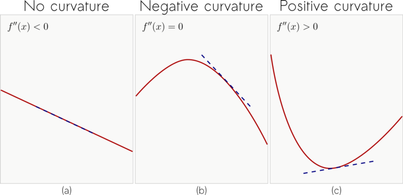
Especially in (c), depending on the magnitude of the step we take, we might get our loss function to rather increasing. To avoid this problem, we take advantage of the information given by the second derivative.

In practice, instead of only taking the derivative of the cross-entropy, we also take the derivative of its derivative. The second derivative, described by f’’(x), gives information about the curvature of a function.

Intuitively, if:

f’’(x)=0, then there is no curvature.
f’’(x)<0, it means that the function curves downward.
f’’(x)>0, there is an upward curvature in the function.

With that information, the update step, for minimizing the cross-entropy takes the form of:

This update equation is called Newton-Raphson.

Note that it multiplies the inverse of the matrix H⁻¹ by the gradient. H, or the Hessian, stores the second derivatives of the cross-entropy w.r.t the weights w.

Let’s now dive into the code.

Taking this toy dataset as an example.

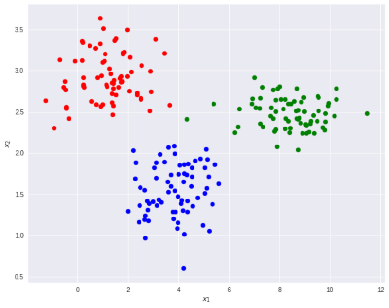
There are 210 points in this 2D coordinate system with 3 classes: blue, red and green circles. Since the number of classes is greater than 2, we can use Softmax Logistic Regression.

First, to introduce the bias variables to our model, we can perform a simple transformation called: fixed basis function. This is done by simply adding a column full of 1s to the input. For binary classification, it makes the corresponding weight value w₀ to play the role of the bias. For multiclass, the first column of the weight matrix act as the biases.

Then, we can create a Logistic Regression object.

Following sklearn’s based API, we can fit and evaluate the model

Note that we can choose between Newton’s and Gradient descent update rules. While Newton’s method tends to converge faster, it needs to compute and store a full Hessian in each iteration. Besides, the Hessian needs to be invertible — for parameter update.

For a matrix to be invertible, there are some constraints that must be true.

First, H has to be a square matrix. Second, the columns of H need to be linearly independent. It means that for any column i of H, i cannot be represented as a linear combination of any other column j.

Since for really large matrices these constraints are likely not to hold, we can use pseudo-inverse techniques here. That is what the function pinv(H) does on the code below.

That is the same to say that the columns of H span the coordinate system. Or that the determinant of H is non-zero.

Even though for smaller datasets, this might not be a problem, the Hessian tends to grow as the number of feature and classes increase. To have an idea, using inputs with M features and a dataset with K classes. The full Hessian has shape [MK, MK]; which for this example mean: [9x9] — remember, we added a new feature column to the inputs.

For the CIFAR-10 dataset, each RGB image has a shape of 32x32x3. That means storing and inverting a square matrix of shape [30720x30720]. Using float 32-bit precision, the Hessian requires 3.775 GB (gigabytes).

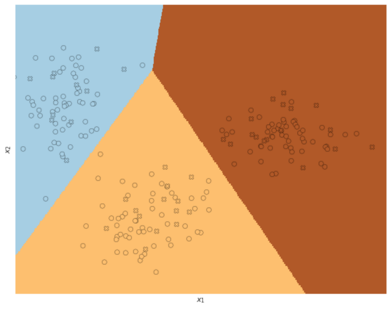
To close up, have a look at the fitted model using the toy dataset and Newton’s method. The crosses are the test data.

Enjoy.

In summary, generative models are a class of ML algorithms that learn the class probabilities explicitly.

They usually perform well with fewer training examples.
They can deal with missing data.
Can be used for supervised and unsupervised learning.

Discriminative models learn the class probabilities implicitly.

In general, they require more labeled data.
They often have fewer assumptions and fewer parameters.
But, can only be used for supervised training.

For binary classification, Logistic Regression uses the sigmoid function to represent the posterior probabilities. For multiclass classification, it uses softmax.

Thanks for reading!

Cite as:

@article{
  silva2019logisticregression,
  title={Logistic Regression: The good parts},
  author={Silva, Thalles Santos},
  journal={https://sthalles.github.io},
  year={2019}
  url={https://sthalles.github.io/logistic-regression/}
}