Practical Deep Learning Audio Denoising

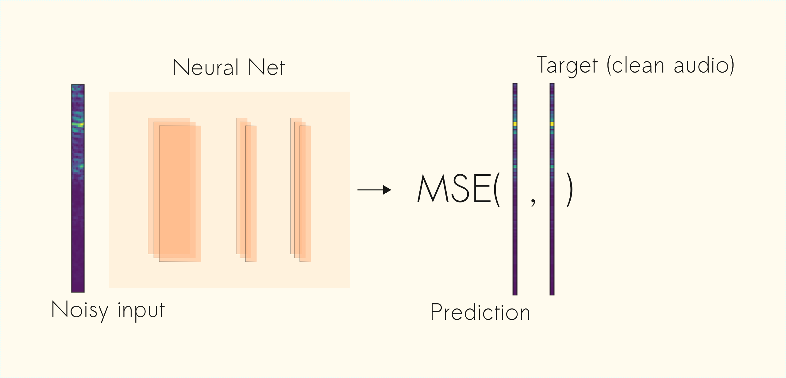
Introduction

Speech denoising is a long-standing problem. Given an input noisy signal, we aim to filter out the undesired noise without degrading the signal of interest. You can imagine someone talking in a video conference while a piece of music is playing in the background. In this situation, a speech denoising system has the job of removing the background noise in order to improve the speech signal. Besides many other use cases, this application is especially important for video and audio conferences where noise can significantly decrease speech intelligibility.

Classical solutions for speech denoising usually use generative modeling. The idea is to use statistical methods like Gaussian Mixtures, to build a model of the noise of interest. Then, we can use it to recover the source (clean) audio from the input noisy signal. However, recent development has shown that in situations where data is plenty available, deep learning often outperforms such solutions.

In this article, we tackle the problem of speech denoising using Convolutional Neural Networks (CNNs). Given a noisy input signal, we aim to build a statistical model that can extract the clean signal (the source) and return it to the user. Here, we focus on source separation of regular speech signals from 10 different types of noise often found in an urban street environment.

You can check out the complete implementation on my GitHub.

The Data

We used 2 popular publicly available audio datasets.

• The Mozilla Common Voice (MCV)
• The UrbanSound8K dataset

As Mozilla puts it on the MCV website:

Common Voice is Mozilla’s initiative to help teach machines how real people speak.

The dataset contains as many as 2,454 recorded hours spread in short MP3 files. The project is open source and anyone can collaborate with it. Here, we used the English portion of the data which contains 30GB of 780 validated hours of speech. One very good characteristic of this dataset is the vast variability of speakers. It contains snippets of men and women recordings from a large variety of ages and foreign accents.

The UrbanSound8K dataset also contains small snippets (<=4s) of sounds. However, these are 8732 labeled examples of 10 different commonly found urban sounds. The complete list includes:

• 0 = air_conditioner
• 1 = car_horn
• 2 = children_playing
• 3 = dog_bark
• 4 = drilling
• 5 = engine_idling
• 6 = gun_shot
• 7 = jackhammer
• 8 = siren
• 9 = street_music

As you might be imagining at this point, we are going to use the urban sounds as noise signals to the speech examples. In other words, we first take a small speech signal – this can be someone speaking a random sentence from the MCV dataset. Then, we add noise to it – you can imagine a woman speaking and a dog backing on the background. Finally, we use this artificially noised signal as the input to our deep learning model. The Neural Net, in turn, receives this noisy signal and tries to output a clean representation of it.

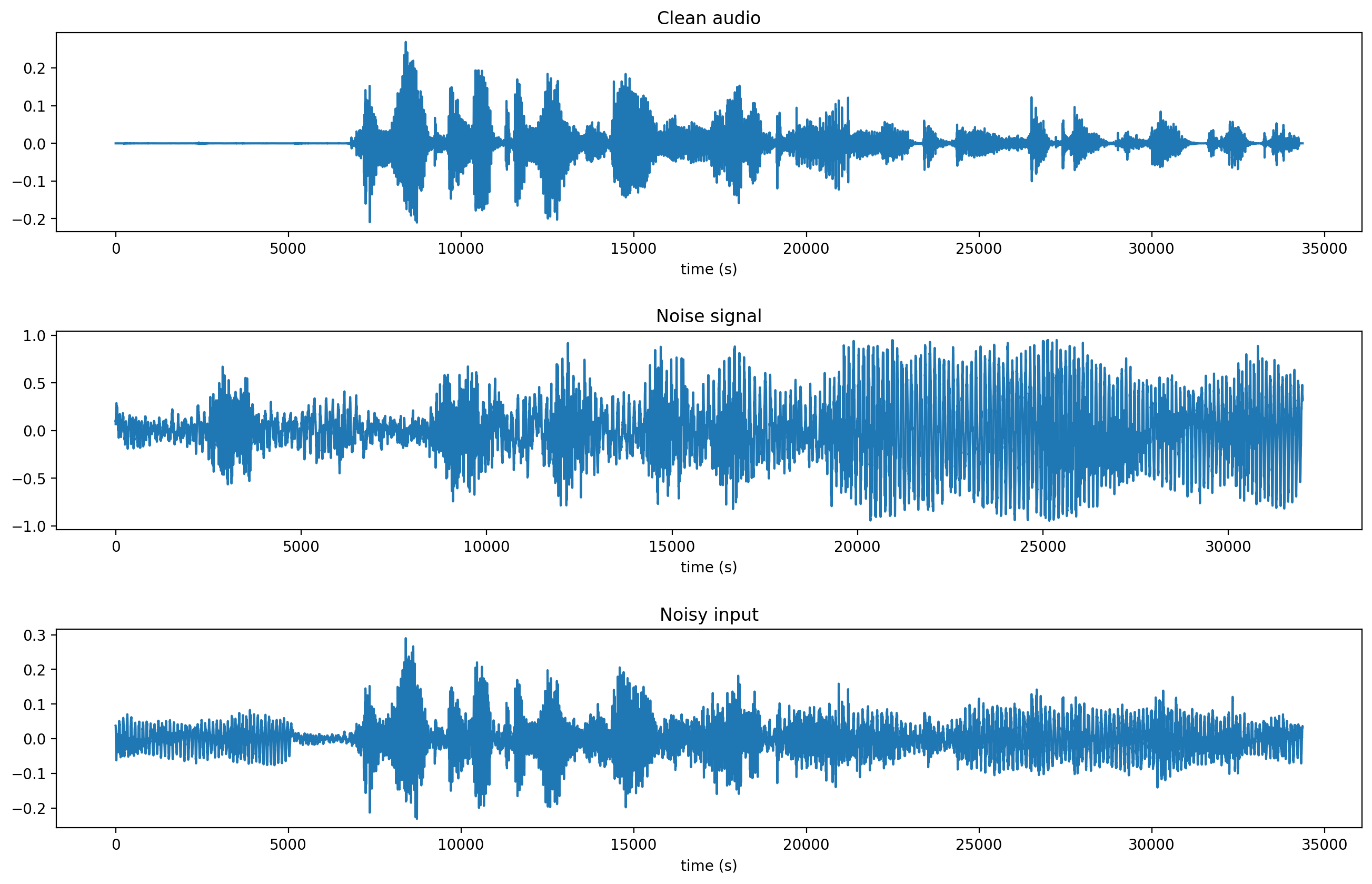
The image below displays a visual representation of a clean input signal from the MCV (top). A noise signal from the UrbanSound dataset (middle) and the resulting noise input – that is the input speech after adding noise to it. Also, note that the noise power is set so that the signal-to-noise ratio (SNR) is zero dB (decibel).

Data Preprocessing

Most of the benefits of current deep learning systems rest in the fact that hand-crafted features ceased to be an essential step to build a state of the art model. Take feature extractors like SIFT and SURF as an example. Those are/were often used in Computer Vision problems like panorama stitching. These methods extract features from local parts of an image to construct an internal representation of the image itself. However, to achieve the necessary goal of generalization, a vast amount of work was necessary to create features that were robust enough to real-world scenarios. Put differently, these features needed to be invariant to common transformations that we often see day-to-day. Those might include variations in rotation, translation, scaling, and so on. And despite the hard work put into creating generalizable feature extractors like BRISK and ORB, this task is not pleasant.

However, one of the cool things about current deep learning is that most of these properties are learned either from the data and/or from special operations like the convolution.

For audio processing, we also hope that the Neural Net will extract relevant features from the data. However, before feeding the raw signal to the network, we need to get it into the right format.

Before we begin, we first downsampled the audio signals (from both datasets) to 8kHz, and removed the silent frames from them. The goal is to reduce the amount of computation and dataset size.

It is important to note that audio data differ from images. Since one of our assumptions is to use CNNs (originally designed for Computer Vision), it is important to be aware of such subtle differences. Audio data, in its raw form, is a 1-dimensional time-series data. Images, on the other hand, are 2-dimensional representations of an instant moment in time. For these reasons, audio signals are often transformed into (time/frequency) 2D representations.

The Frequency Cepstral Coefficients (MFCCs) and the constant-Q spectrum are 2 of the most popular representations used on audio applications. For deep learning though, we may avoid classic MFCCs because they remove a lot of information and do not preserve spatial relations–this is especially important for audio reconstruction. Additionally, source separation tasks are often done in the time-frequency domain.

Another important point is that audio signals are, in their majority, non-stationary. In other words, the signal’s mean and variance are not constant over time. Thus, there is not much sense in computing a Fourier Transform over the entire audio signal. For this reason, we feed the DL system with spectral magnitude vectors computed using a 256-point Short Time Fourier Transform (STFT).

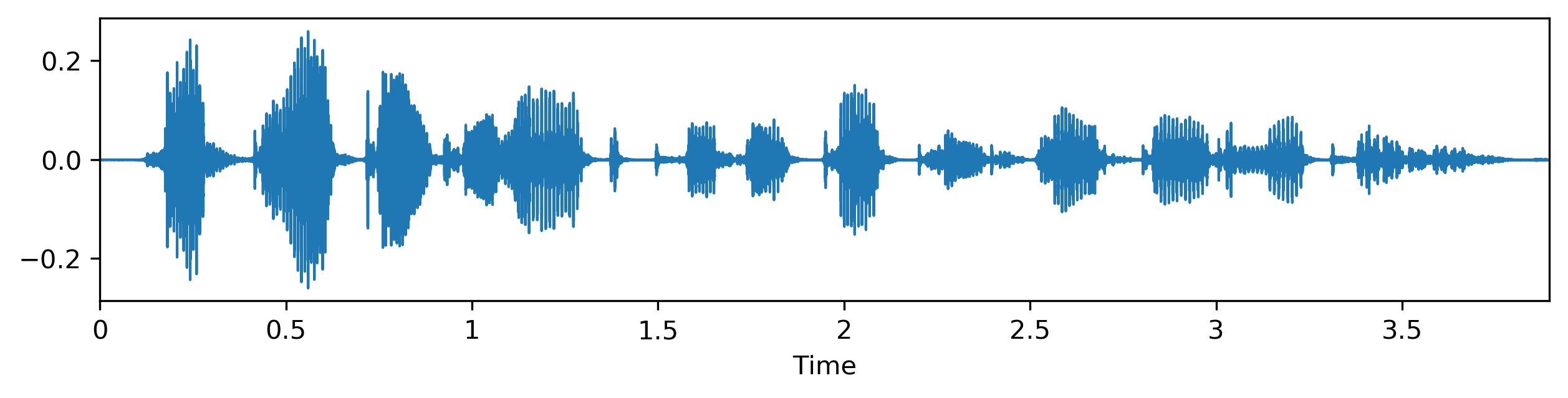
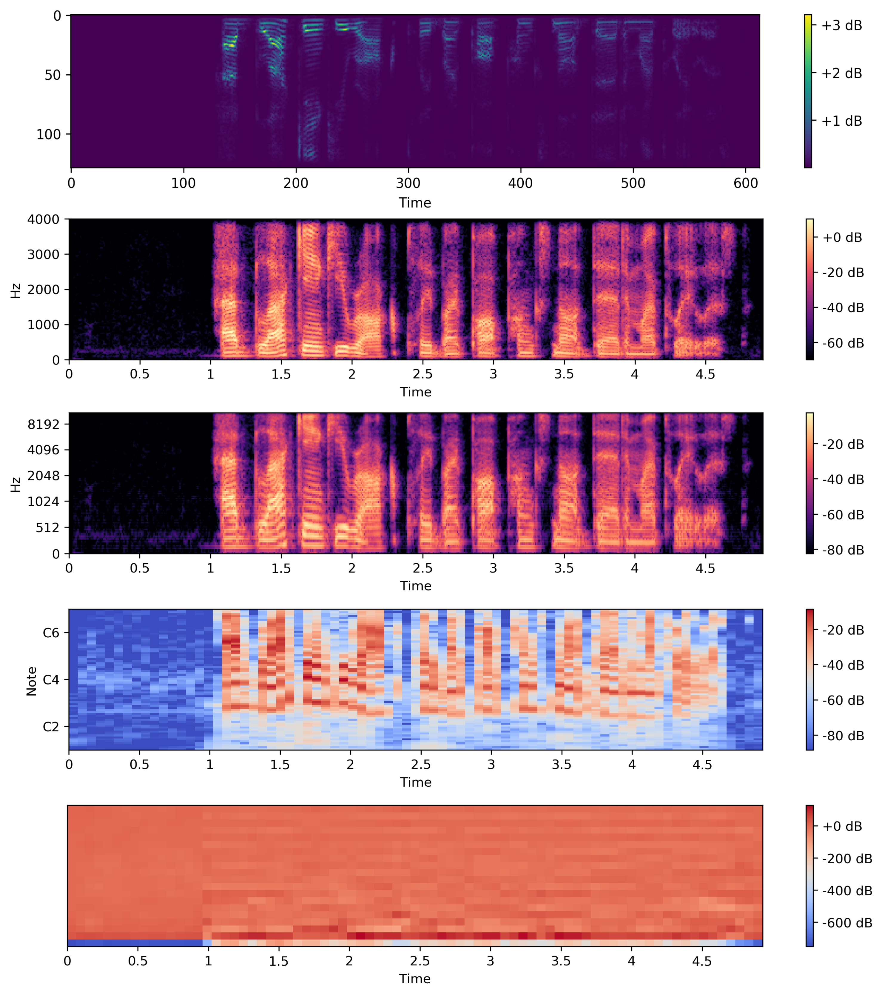
You can see bellow, common representations of audio signals.

To calculate the STFT of a signal, we need to define a window of length M and a hop size value R. The latter defines how the window moves over the signal. Then we slide the window over the signal and calculate the discrete Fourier Transform (DFT) of the data within the window. Thus, the STFT is simply the application of the Fourier Transform over different portions of the data. Lastly, we extract the magnitude vectors from the 256-point STFT vectors and take the first 129-point by removing the symmetric half. All this process was done using the Python Librosa library. The image below from MATLAB, illustrates the process.

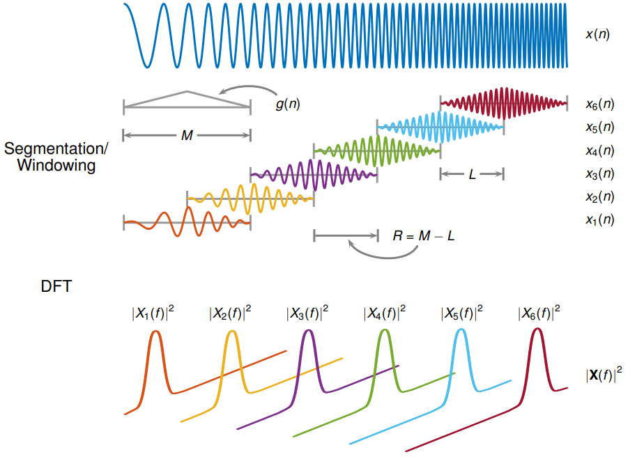
Image Credits to: MATLAB STFT docs.

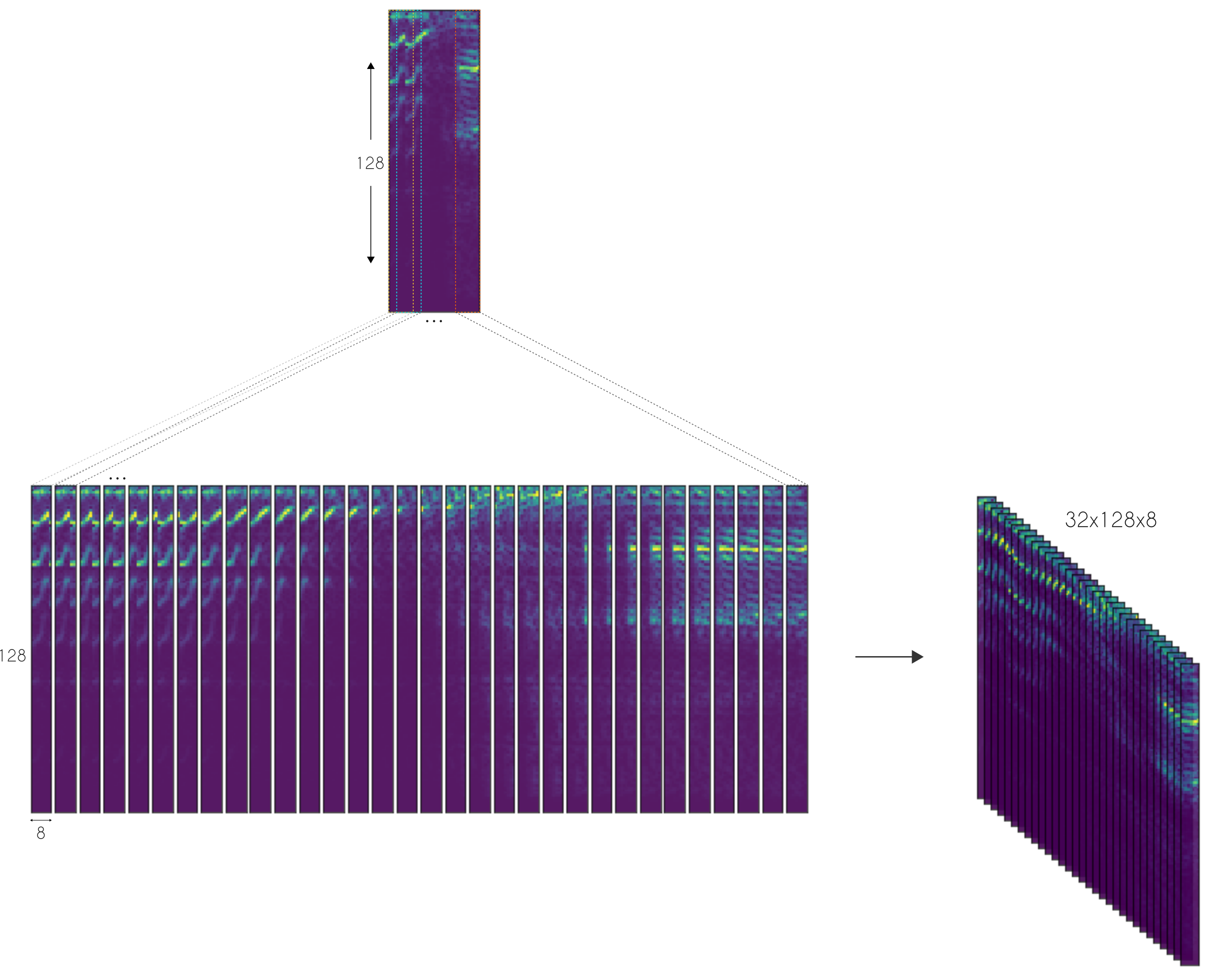
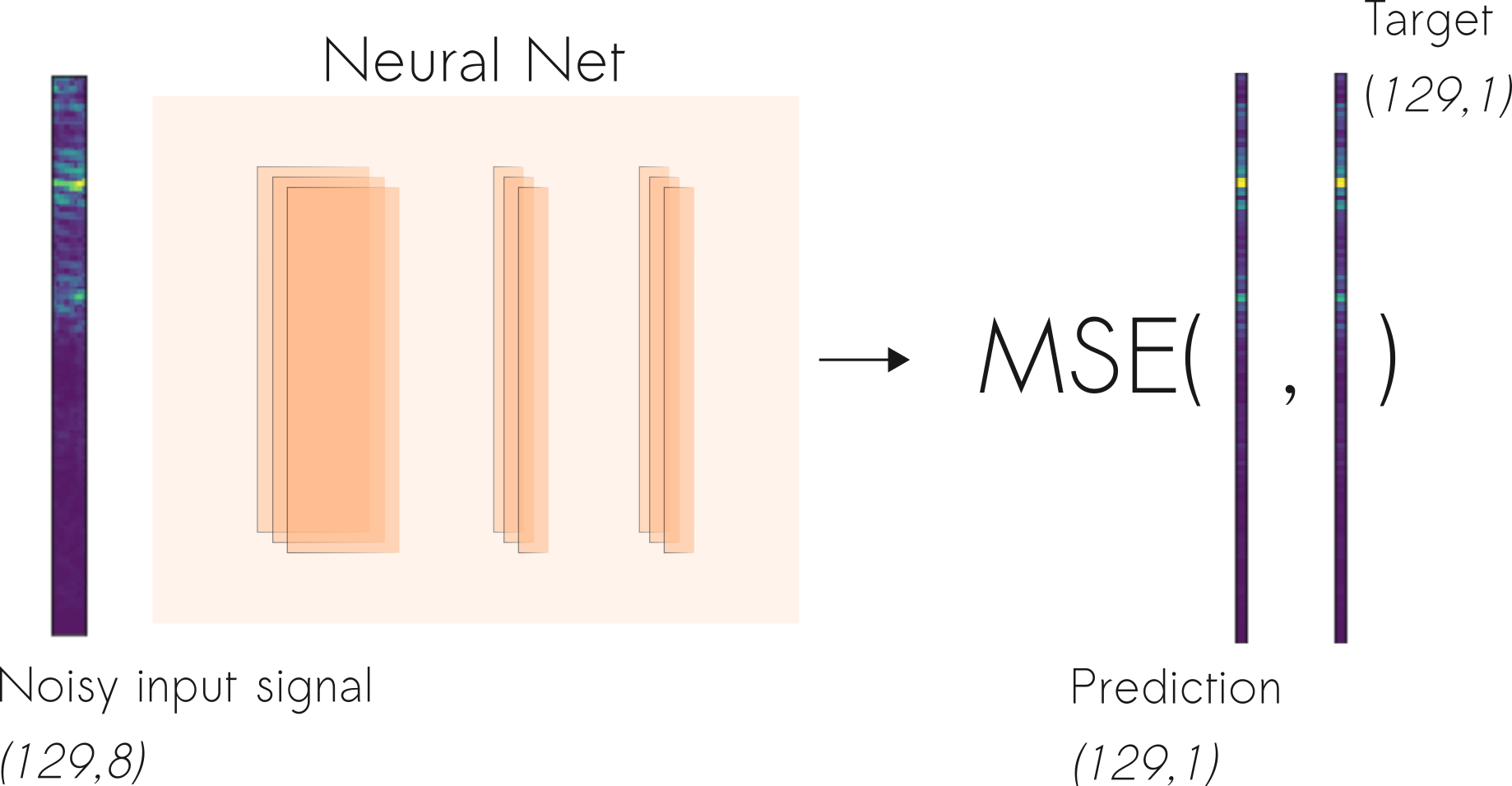
Here, we defined the STFT window as a periodic Hamming Window with length 256 and hop size of 64. This ensures a 75% overlap between the STFT vectors. In the end, we concatenate 8 consecutive noisy STFT vectors and use them as inputs. Thus, an input vector has a shape of (129,8) and is composed of the current STFT noise vector plus 7 previous noise STFT vectors. In other words, the model is an autoregressive system that predicts the current signal based on past observations. Therefore, the targets consist of a single STFT frequency representation of shape (129,1) from the clean audio.

Deep Learning Architecture

Our Deep Convolutional Neural Network (DCNN) is largely based on the work done by A fully convolutional neural network for speech enhancement. Here, the authors propose the Cascaded Redundant Convolutional Encoder-Decoder Network (CR-CED).

The model is based on symmetric encoder-decoder architectures. Both components contain repeated blocks of Convolution, ReLU and Batch Normalization. In total, the network contains 16 of such blocks, which add up to 33K parameters.

Also, there are skip connections between some of the encoder and decoder blocks. Here the feature vectors from both components are combined through addition. Very much like ResNets, the skip connections speed up convergence and reduces the vanishing of gradients.

Another important characteristic of the CR-CED network is that convolution is only done in 1 dimension. More specifically, given an input spectrum of shape (129 x 8), convolution is only performed in the frequency axis (i.e the first one). This ensures that the frequency axis remains constant during forwarding propagation.

The combination of a small number of training parameters and model architecture makes this model a lightweight option for fast execution on mobile or edge devices.

Once the network produces an output estimate, we optimize (minimize) the mean squared difference (MSE) between the output and the target (clean audio) signals.

Results and Discussion

Let’s check some of the results achieved by the CNN denoiser.

To begin, listen to test examples from the MCV and UrbanSound datasets. They are the clean speech and noise signal respectively. To recap, we use the clean signal as the target and the noise audio as the source of the noise.

Now, take a look at the noise signal passed as input to the model and the respective denoised result.

Below, you can compare the denoised CNN estimation (bottom) with the target (clean signal on the top) and noise signal (used as input in the middle).

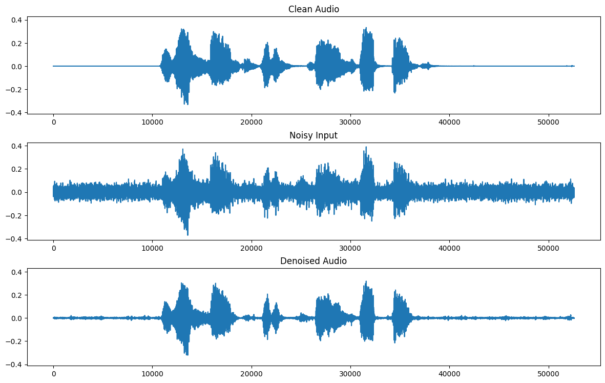
As you can see, given the difficulty of the task, the results are somewhat acceptable but not perfect. Indeed, in most of the examples, the model manages to smooth the noise but it doesn’t get rid of it completely.

Take a look at a different example, this time with a dog barking in the background.

One of the reasons that prevent better estimates is the loss function. The Mean Squared Error (MSE) cost, optimizes the average over the training examples. We can think of it as finding the mean model that smooths the input noise audio to provide an estimate of the clean signal. Thus, one of the solutions is to devise more specific loss functions to the task of source separation.

A particularly interesting possibility is to learn the loss function itself using GANs (Generative Adversarial Networks). Indeed, we could frame the problem of audio denoising as a signal-to-signal translation problem. Very much like image-to-image translation, first, a Generator network receives a noise signal and outputs an estimate of the clean signal. Then, the Discriminator net receives the noise input as well as the generator predictor or the real target signals. This way, the GAN will be able to learn the appropriate loss function to map input noisy signals to their respective clean counterparts. That is an interesting possibility that I look forward to implementing.

Thanks for reading!

Cite as:

@article{
  silva2019audiodenoising,
  title={Practical Deep Learning Audio Denoising},
  author={Silva, Thalles Santos},
  journal={https://sthalles.github.io},
  year={2019}
  url={https://sthalles.github.io/practical-deep-learning-audio-denoising/}
}