Semi-supervised Learning with GANs
[machine-learning deep-learning representation-learning semi-supervised-learning tensorflow python gans generative-models 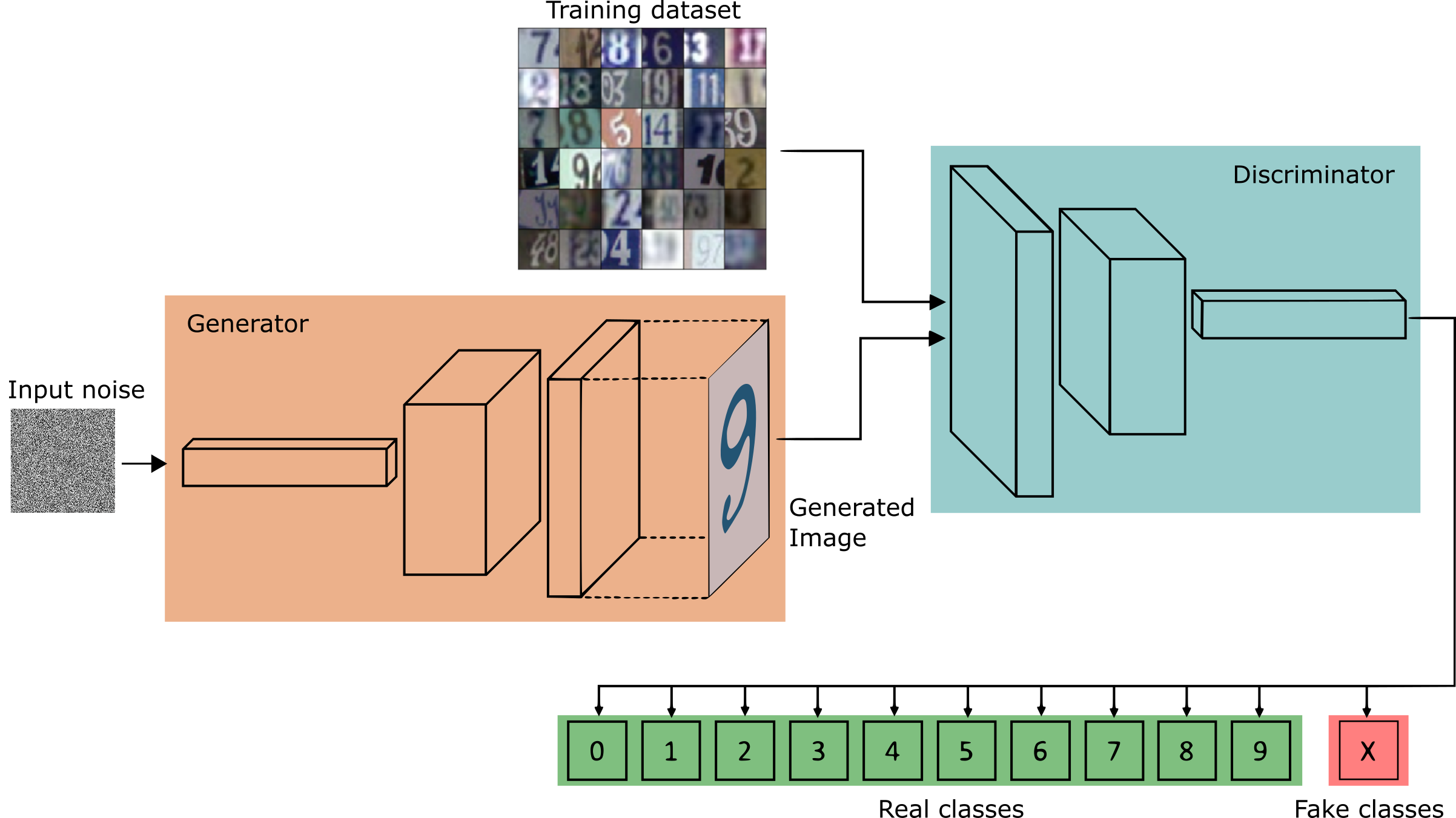
Intro
Note, since some of the content of A Short Introduction to Generative Adversarial Networks is mentioned here, I recommend you to have a look at it before reading this peace for a clearer understanding.
In the previous blog post, we talked about the intuition behind GANs (Generative Adversarial Networks), how they work, and how to create a simple GAN model capable of learning how to generate images that look a lot like images from the MNIST and SVHNs datasets. Now, let us turn the wheels a little and talk about one of the most prominent applications of GANs, semi-supervised learning.
If you ever heard or studied about deep learning before, you probably have heard about MNIST, SVHN, ImageNet, PascalVoc and others. All of these datasets have one thing in common, each of them consists of hundreds and thousands of labeled data. That is, all of these collections of data are composed of (x,y) pairs where (x) is the raw data, an image matrix for instance, and (y) is a description of what that data point (x) represents.
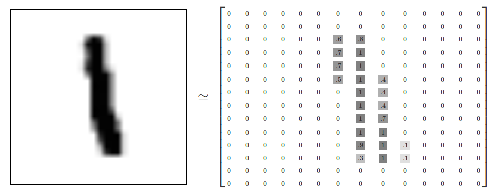
Take the MNIST dataset as an example, each of the 60,000 data points can be viewed as an (image, label) pair where image is a 28x28 grayscale image tensor and label is an indication of weather that image represents a one, two or three and so on up to nine possible categories.
The most common usage of such datasets is to develop supervised models. To train such algorithms, we usually provide a tremendous amount of data examples with labels so that the model can learn the structure of these datasets and after training, they become able to take consistent decisions even when similar but unseen situations come around.
Think of that as a professor teaching a kid how to spell the word “learning”. At first, the kid probably will get it wrong and write something like “learneng” for instance. That is where the supervision/teacher comes into play showing that the correct spelling is “learning”, so the kid next time will have a much higher chance of spelling it correctly.
Supervised learning has been the center of most researching in deep learning in recent years. However, the necessity of creating models capable of learning from fewer or no labeled data is greater year by year.
With that in mind, the technique in which both labeled and unlabeled data is used to train a machine learning classifier is called semi-supervised learning. Typically, a semi-supervised classifier takes a tiny portion of labeled data and a much larger amount of unlabeled data (from the same domain) and the goal is to use both, labeled and unlabeled data to train a neural network to learn an inferred function that after training, can be used to map a new datapoint to its desirable outcomes.
In this frontier, we are going to take the knowledge from the previous post and build a GAN that is able to learn how to classify street view house numbers using only roughly 1.3% of the original SVHN training labels i.e. 1000 (one thousand) labeled examples. We are going to use some of the techniques described in the paper Improved Techniques for Training GANs from OpenAI. The complete code notebook can found here.
Intuition
As you might recall, when building a GAN for generating images, we trained both, the generator and the discriminator simultaneously, and by the end of training, we could discard the discriminator because we used it just for training the generator.
For Semi-supervised learning, we need to transform the discriminator into a multi class classifier that also has to be able to learn how to classify the dataset categories using only a very small portion of the labels. Taking the SVHN dataset as the training case, we are going to use only 1000 labeled examples (out of the 73257 training labels) and use the rest as unsupervised data to help training the classifier.
In addition, this time, by the end of training, we can actually throw away the generator because now, we use the generator only for guiding the discriminator during training. That is to say, the generator now acts as a different source of information for which the discriminator gets raw unlabeled images from in order to improve its performance.
For a regular image generation GAN, the discriminator has only one role, which is to compute the probability of whether its inputs are real or not, let us call it the GAN problem. However, to turn the discriminator into a semi-supervised classifier, in addition to the GAN problem, the discriminator has also to learn the probabilities of each of the original dataset classes it is trained on.
Recall that for the discriminator output we showed in the previous blog post, we have a single sigmoid unit that represents the probability of an input image being real (value close to 1 - coming from the training set), or fake (value close to 0 - coming from the generator net). That probability is important because by using it, the discriminator is able to send a signal back to the generator that makes it possible to improve the generator’s capabilities of creating realistic images.
This time, the discriminator still has to send its gradients back to the generator, since that is the only source of information the generator has to adapt its parameters during training. However, in case of real images, the discriminator also has to output individual probabilities for each of the individual dataset classes.
To do that, we can turn the sigmoid output (from the previous GAN) into a softmax with 11 class outputs, the first 10 for the individual class probabilities of the SVHN dataset (zero to nine), and the 11th class for all the fake images that come from the generator. Note that if we set the 11th class probability to 0, then the sum of the 10 probabilities represents the same probability previously computed using the sigmoid function.
Lastly, we need to setup the losses in such a way that the discriminator can do both (1) help the generator learn to produce realistic images, that is done by learning to distinguish between real and fake samples, and (2) use the generator’s images along with the labeled and unlabeled training images to precisely classify the datasets categories.
To summarize, the discriminator has three different sources of input data for training.
- Real images with labels; on these we provide image label pairs just like in any regular supervised classification problem.
- Real images without labels; for those, the classifier only learns that these images are real.
- Images from the generator; to these ones, the discriminator learns to classify as fake.
The insight is that the combination of all of these sources of data will make the classifier able to learn from a much broader perspective making it able to determine the correct outcome much more precisely than it would be if only using the 1000 labeled examples.
Generator
The Generator follows a very standard implementation described in the DCGAN paper. This approach consists of reshaping a random vector z to have a 4D shape and then feed it to a sequence of transpose convolutions, batch normalization and leaky RELU operations that increase the spatial dimensions of the input vector while decreases the number of channels. As a result, the network outputs a 32x32x3 RGB tensor shape that is squashed between values of -1 and 1 through the Hyperbolic Tangent Function.
def generator(z, output_dim, reuse=False, alpha=0.2, training=True, size_mult=128):
    with tf.variable_scope('generator', reuse=reuse):
        # First fully connected layer
        x1 = tf.layers.dense(z, 4 * 4 * size_mult * 4)
        # Reshape it to start the convolutional stack
        x1 = tf.reshape(x1, (-1, 4, 4, size_mult * 4))
        x1 = tf.layers.batch_normalization(x1, training=training)
        x1 = tf.maximum(alpha * x1, x1)

        x2 = tf.layers.conv2d_transpose(x1, size_mult * 2, 5, strides=2, padding='same')
        x2 = tf.layers.batch_normalization(x2, training=training)
        x2 = tf.maximum(alpha * x2, x2)

        x3 = tf.layers.conv2d_transpose(x2, size_mult, 5, strides=2, padding='same')
        x3 = tf.layers.batch_normalization(x3, training=training)
        x3 = tf.maximum(alpha * x3, x3)

        # Output layer
        logits = tf.layers.conv2d_transpose(x3, output_dim, 5, strides=2, padding='same')

        out = tf.tanh(logits)

        return out
Discriminator
The discriminator, now a multi class classifier, is the most relevant network for this architecture. Here we setup an also similar DCGAN architecture in which we use a stack of strided 2 convolutions for dimensionality reduction and batch normalization for stabilizing learning (except for the first layer of the network).
The 2D convolution window (kernel or filter) is set to have a width and height of 3 across all the convolution operations. Also, note that we have some layers with dropout. It is important to understand that our discriminator behaves (in part) like any other regular classifier and because of that; it may suffer from the same problems any classifier would if not well designed.
One of the most likely drawback one might encounter when training a big classifier on a very limited labeled dataset is the imminence of overfitting. One thing to watch on “over trained” classifiers is that they typically show a notably difference between the training error (smaller) and the testing error (higher). This situation shows that the model did a good job capturing the structure of the training dataset but at the same time, because the model believed too much in the training data, it fails to generalize what it has learned for unseen examples. To prevent that, we make an extensive usage of dropout even for the first layer of the network.
def discriminator(x, reuse=False, alpha=0.2, drop_rate=0., num_classes=10, size_mult=64):
    with tf.variable_scope('discriminator', reuse=reuse):
        x = tf.layers.dropout(x, rate=drop_rate/2.5)

        # Input layer is ?x32x32x3
        x1 = tf.layers.conv2d(x, size_mult, 3, strides=2, padding='same')
        relu1 = tf.maximum(alpha * x1, x1)
        relu1 = tf.layers.dropout(relu1, rate=drop_rate) # [?x16x16x?]

        x2 = tf.layers.conv2d(relu1, size_mult, 3, strides=2, padding='same')
        bn2 = tf.layers.batch_normalization(x2, training=True) # [?x8x8x?]
        relu2 = tf.maximum(alpha * bn2, bn2)

        x3 = tf.layers.conv2d(relu2, size_mult, 3, strides=2, padding='same') # [?x4x4x?]
        bn3 = tf.layers.batch_normalization(x3, training=True)
        relu3 = tf.maximum(alpha * bn3, bn3)
        relu3 = tf.layers.dropout(relu3, rate=drop_rate)

        x4 = tf.layers.conv2d(relu3, 2 * size_mult, 3, strides=1, padding='same') # [?x4x4x?]
        bn4 = tf.layers.batch_normalization(x4, training=True)
        relu4 = tf.maximum(alpha * bn4, bn4)

        x5 = tf.layers.conv2d(relu4, 2 * size_mult, 3, strides=1, padding='same') # [?x4x4x?]
        bn5 = tf.layers.batch_normalization(x5, training=True)
        relu5 = tf.maximum(alpha * bn5, bn5)

        x6 = tf.layers.conv2d(relu5, 2 * size_mult, 3, strides=2, padding='same') # [?x2x2x?]
        bn6 = tf.layers.batch_normalization(x6, training=True)
        relu6 = tf.maximum(alpha * bn6, bn6)
        relu6 = tf.layers.dropout(relu6, rate=drop_rate)
...
After a series of convolutions, batch normalization, leaky RELUs and dropout, instead of directly applying a fully connected layer on top of the convolutions, we perform a Global Average Pooling (GAP) operation. Global Average Pooling is a regularization technique that has been used with success in some convolutional classifier nets as a replacement to fully connected layers. In GAP we take the average over the spatial dimensions of a feature map resulting in one value.
...
# Flatten it by global average pooling
# In global average pooling, for every feature map we take the average over all the spatial
# domain and return a single value
# In: [BATCH_SIZE,HEIGHT X WIDTH X CHANNELS] --> [BATCH_SIZE, CHANNELS]
features = tf.reduce_mean(relu7, axis=[1,2])

# Set class_logits to be the inputs to a softmax distribution over the different classes
class_logits = tf.layers.dense(features, num_classes)
...
For instance, suppose that after a series of convolutions, we get a tensor of shape [BATCH_SIZE, 8, 8, CHANNELS] and we want to apply GAP to flat this feature map. GAP works by taking the average value over the [8x8] tensor slice resulting in a tensor of shape [BATCH_SIZE, 1, 1, CHANNELS] that can be reshaped to [BATCH_SIZE, CHANNELS].
In Network in network, the authors describe several advantages over traditional fully connected layers such as a higher robustness for spatial translation of the input and less overfitting concerns. After the GAP operation, a fully connected layer is applied to output a feature map that corresponds to the number of classes we want to predict.
Once we get logits associated with the different classes, putting these logits through a softmax gives us the classification probabilities over the classes we want to predict. However, we still need a way to represent the probability of an input image being real rather than fake, that is, we still need to model the binary classification problem for a regular GAN model.
...
# Get the probability that the input is real rather than fake
out = tf.nn.softmax(class_logits) # class probabilities for the 10 real classes
...
We can think that the logits are in terms of softmax logits and we need to represent them as sigmoid logits as well. Given that the probability of an input being real corresponds to the sum over the real class logits, we can feed these values into a LogSumExp function that will model the binary classification value to be fed to a sigmoid function. In order to avoid numerical stabilization problems with the LogSumExp function, we can use the Tensorflow built-in function that will prevent numerical issues that may occur when LogSumExp encounters very extreme either positive or negative values.
...
# This function is more numerically stable than log(sum(exp(input))).
# It avoids overflows caused by taking the exp of large inputs and underflows
# caused by taking the log of small inputs.
gan_logits = tf.reduce_logsumexp(class_logits, 1)
...
Model Loss
We can divide the discriminator loss into two parts, one that represents the GAN problem, or the unsupervised loss, and the other that computes the individual real class probabilities, the supervised loss.
For the unsupervised loss, as we mentioned, the discriminator still has to differentiate between real training images and fake images from the generator. As for a regular GAN, half of the time the discriminator receives unlabeled images from the training set and the other half, imaginary unlabeled images from the generator. Since in both cases we are dealing with a binary classification problem in which we want a probability value near 1 for real images and near 0 for unreal images, we use the sigmoid cross entropy function to compute the loss.
For images coming from the training set, we maximize their probabilities of being real by assigning labels of 1s, and for fabricated images coming from the generator, we maximize their probabilities to be fake by giving them labels of 0s.
...
# Here we compute `d_loss`, the loss for the discriminator.
# This should combine two different losses:
# 1. The loss for the GAN problem, where we minimize the cross-entropy for the binary
#    real-vs-fake classification problem.
tf.reduce_mean(tf.nn.sigmoid_cross_entropy_with_logits(logits=gan_logits_on_data,
                                                        labels=tf.ones_like(gan_logits_on_data) * (1 - smooth)))

fake_data_loss = tf.reduce_mean(tf.nn.sigmoid_cross_entropy_with_logits(logits=gan_logits_on_samples,
                                                     labels=tf.zeros_like(gan_logits_on_samples)))

# This way, the unsupervised
unsupervised_loss = real_data_loss + fake_data_loss
...
For the supervised loss, we need to use the logits from the discriminator, and since this is a multiclass classification problem, we perform a softmax cross entropy using the real labels we have available. Note that this part is similar to any other classification model. In the end, the discriminator loss is the sum of both the supervised loss and the unsupervised loss. Also, note that because we are pretending we do not have most of the labels, we need to ignore them in the supervised loss. To do that, we just multiply the loss by the masks variable that basically indicates which set of labels are available for usage.
#  2. The loss for the SVHN digit classification problem, where we minimize the cross-entropy
#     for the multi-class softmax. For this one we use the labels. Don't forget to ignore
#     use `label_mask` to ignore the examples that we are pretending are unlabeled for the
#     semi-supervised learning problem.
y = tf.squeeze(y)
suppervised_loss = tf.nn.softmax_cross_entropy_with_logits(logits=class_logits_on_data,
                                                              labels=tf.one_hot(y, num_classes, dtype=tf.float32))

label_mask = tf.squeeze(tf.to_float(label_mask))

# ignore the labels that we pretend does not exist for the loss
suppervised_loss = tf.reduce_sum(tf.multiply(suppervised_loss, label_mask))

# get the mean
suppervised_loss = suppervised_loss / tf.maximum(1.0, tf.reduce_sum(label_mask))
d_loss = unsupervised_loss + suppervised_loss
For the generator loss, as described in the Improved Techniques for Training GANs paper, we use feature matching. As the authors describe, feature matching is the concept of “penalizing the mean absolute error between the average value of some set of features on the training data and the average values of that set of features on the generated samples”.
To do that, we take some set of statistics (the moments) from two different sources and force them to be similar. First, we take the average values of the features extracted from the discriminator when a real training minibatch is being processed. Second, we compute the moments in the same way but now for when a minibatch composed of fake images that come from the generator was being analyzed by the discriminator, and finally, with these two sets of moments, the generator loss is the mean absolute difference between them. In other words, as the paper emphasizes, “we train the generator to match the expected values of the features on an intermediate layer of the discriminator”.
# Here we set `g_loss` to the "feature matching" loss invented by Tim Salimans at OpenAI.
# This loss consists of minimizing the absolute difference between the expected features
# on the data and the expected features on the generated samples.
# This loss works better for semi-supervised learning than the tradition GAN losses.
# Make the Generator output features that are on average similar to the features
# that are found by applying the real data to the discriminator
data_moments = tf.reduce_mean(data_features, axis=0)
sample_moments = tf.reduce_mean(sample_features, axis=0)
g_loss = tf.reduce_mean(tf.abs(data_moments - sample_moments))
pred_class = tf.cast(tf.argmax(class_logits_on_data, 1), tf.int32)
eq = tf.equal(tf.squeeze(y), pred_class)
correct = tf.reduce_sum(tf.to_float(eq))
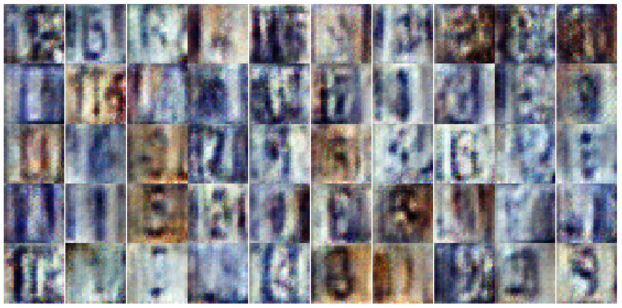
masked_correct = tf.reduce_sum(label_mask * tf.to_float(eq))An interesting curiosity about feature matching is that, although it performs well on the task of semi-supervised learning, you will notice that the images generated by the generator network are not as good as the ones created in the last post.
In the Improved Techniques for Training GANs paper, OpenAI reports state-of-the-art results for semi-supervised classification learning on MNIST, CIFAR-10 and SVHN. This implementation reaches train accuracy of nearly 93% and a test accuracy of roughly 67 to 68%. Although the results might seem good, they are actually a little better than the ones reported in this NIPS 2014 paper which got something around 64%. Note that this notebook is not intended for demonstrating best practices such cross-validation techniques and it only uses some of the techniques described in the paper. The notebook was implemented from the one provided in the Udacity Deep learning Fundamentals nanodegree program in which I am graduated from.
Concluding
As machine learning grows, attempts to solve already establish problems using less labeled data are key for breaking the unsupervised learning obstacles machine learning is facing right now. In this scenario, GANs pose a real alternative for learning complicated tasks with less labeled samples. However, the distance between semi-supervised and fully supervised learning solutions is still far from being equal, but we certainly can expect this gap to become shorter as new approaches come in to play.
Cite as:
@article{
  silva2017semisupervised,
  title={Semi-supervised Learning with GANs},
  author={Silva, Thalles Santos},
  journal={https://sthalles.github.io},
  year={2017}
  url={https://sthalles.github.io/semi-supervised-learning-with-gans/}
}