Exploring SimCLR: A Simple Framework for Contrastive Learning of Visual Representations
[machine-learning deep-learning representation-learning pytorch torchvision unsupervised-learning contrastive-loss simclr self-supervised self-supervised-learning 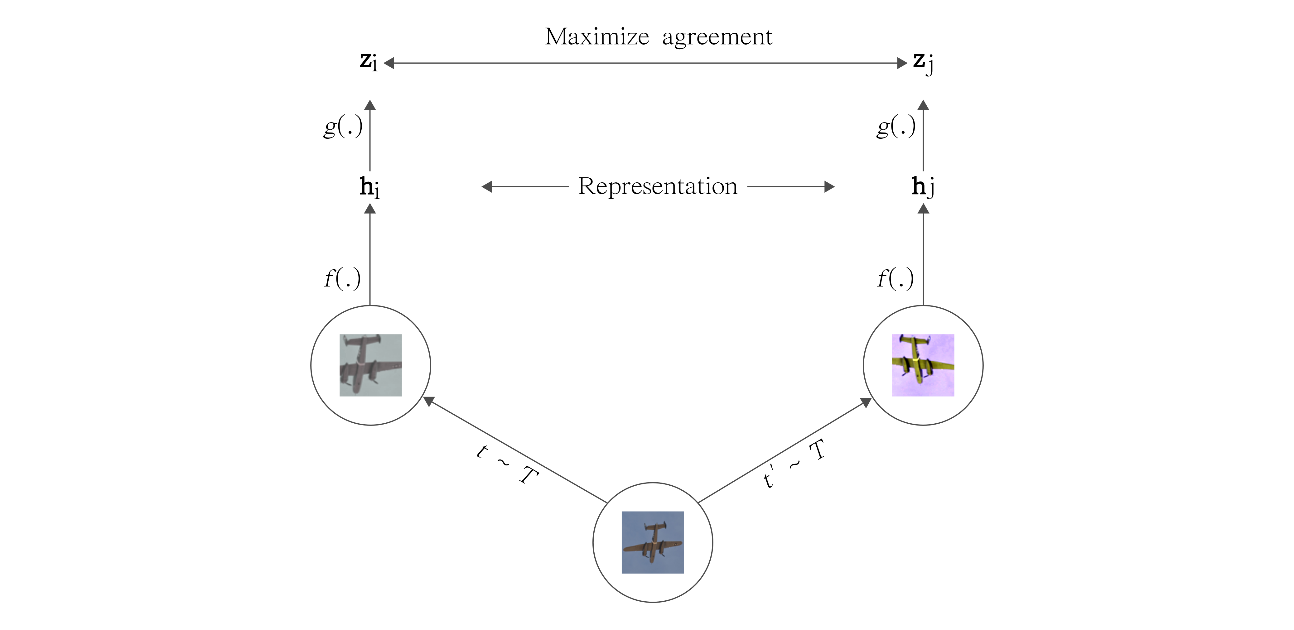
Introduction
For quite some time now, we know about the benefits of transfer learning in Computer Vision (CV) applications. Nowadays, pre-trained Deep Convolution Neural Networks (DCNNs) are the first go-to pre-solutions to learn a new task. These large models are trained on huge supervised corpora, like the ImageNet. And most important, their features are known to adapt well to new problems.
This is particularly interesting when annotated training data is scarce. In situations like this, we take the models’ pre-trained weights, append a new classifier layer on top of it, and retrain the network. This is called transfer learning, and is one of the most used techniques in CV. Aside from a few tricks when performing fine-tuning (if the case), it has been shown (many times) that:
If training for a new task, models initialized with pre-trained weights tend to learn faster and be more accurate then training from scratch using random initialization.
However, as one might guess, there is a bottleneck in this process. Most of the current transfer learning methods rely on models trained on supervised corpora. But the problem is that annotating data is not cheap.
If we look around, data, in an unsupervised way, is abundant. Thus, it makes sense to use unlabeled data to learn representations that could be used as a proxy to achieve better supervised models. In fact, that is a long-standing problem, and current research on unsupervised representation learning is finally catching up with supervised methods.
Unsupervised Representation Learning
Unsupervised representation learning is concerned to address the following issue:
How can we learn good representations from unlabeled data?
Besides the question of what a good representation is, learning from unsupervised data has great potential. It can unlock a number of applications that current transfer learning hasn’t been able to address. Historically, however, unsupervised representation learning has been a much harder problem than its supervised counterpart.
As a simple example, let’s consider the task of breast cancer detection. Currently, all the best solutions use ImageNet pre-trained models as a starting point in the optimization process. Interestingly, even though there is a significant difference between breast cancer slide images and regular ImageNet samples, the transfer learning assumptions still hold to some extent.
To have an idea, most supervised datasets for breast cancer detection, like the CAMELYON dataset, do not compare in size and variability with common Computer Vision supervised datasets. On the other hand, we have a massive number of non-annotated slide images of breast cancer. Thus, if we could learn good representations from the unsupervised (much larger corpora) it would certainly help to learn more specific downstream tasks that have limited annotated data.
Fortunately, visual unsupervised representation learning has shown great promise. More specifically, visual representations learned using contrastive based techniques are now reaching the same level of those learned via supervised methods – in some self-supervised benchmarks.
Let’s explore how unsupervised contrastive learning works and have a closer look at one major work on the area.
Contrastive Learning
Contrastive methods aim to learn representations by enforcing similar elements to be equal and dissimilar elements to be different. In recent months, we have seen an explosion of unsupervised Deep Learning methods based on these principles. In fact, some self-supervised contrastive-based representations already match supervised-based features in linear classification benchmarks.
The core of contrastive learning is the Noise Contrastive Estimator (NCE) loss.

In the equation above, you can think of $x^+$ as a data point similar to the input $x$. In other words, the observations $x$ and $x^+$ are correlated and the pair $(x, x^+)$ represents a positive example. Usually, $x^+$ is the result of some transformation on $x$. This can be a geometric transform aimed to change the size, shape or orientation of $x$, or any type of data augmentation technique. Some examples include rotation, sheer, resize, cutout and more.
On the other hand, $x^-$ are examples dissimilar to $x$. The pair $(x, x^-)$ form a negative example and they are meant to be uncorrelated. Here, the NCE loss will enforce them to be different from the positive pairs. Note that for each positive pair $(x,x^+)$ we have a set of K negatives. Indeed, empirical results have shown that a large number of negatives is required to obtain good representations.
The $sim(.)$ function is a similarity (distance) metric. It is responsible for minimizing the difference between the positives while maximizing the difference between positive and negatives. Often, $sim(.)$ is defined in terms of dot products or cosine similarities.
Lastly, $g(.)$ is a convolution neural network encoder. Specifically, recent contrastive learning architectures use siamese networks to learn embeddings for positive and negative examples. These embeddings are then passed as input to the contrastive loss.
In simple terms, we can think of the contrastive task as trying to identify the positive example among a bunch of negatives.
A Simple Framework for Contrastive Learning of Visual Representations - SimCLR
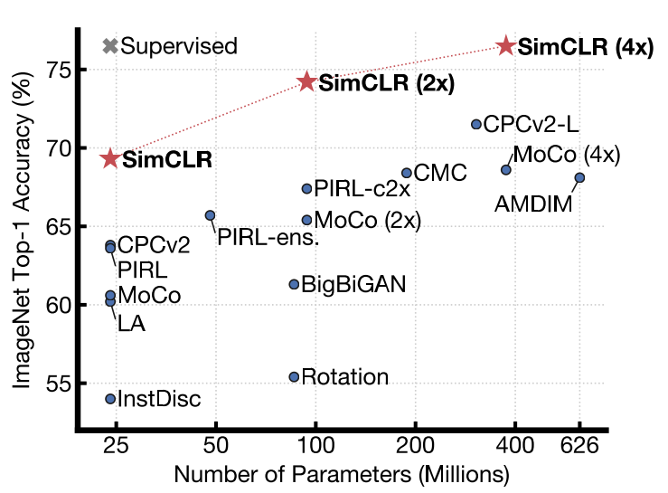
SimCLR uses the same principles of contrastive learning described above. In the proposed paper, the method achieves SOTA in self-supervised and semi-supervised learning benchmarks. It introduces a simple framework to learn representations from unlabeled images based on heavy data augmentation. To put it simply, SimCLR uses contrastive learning to maximize agreement between 2 augmented versions of the same image.
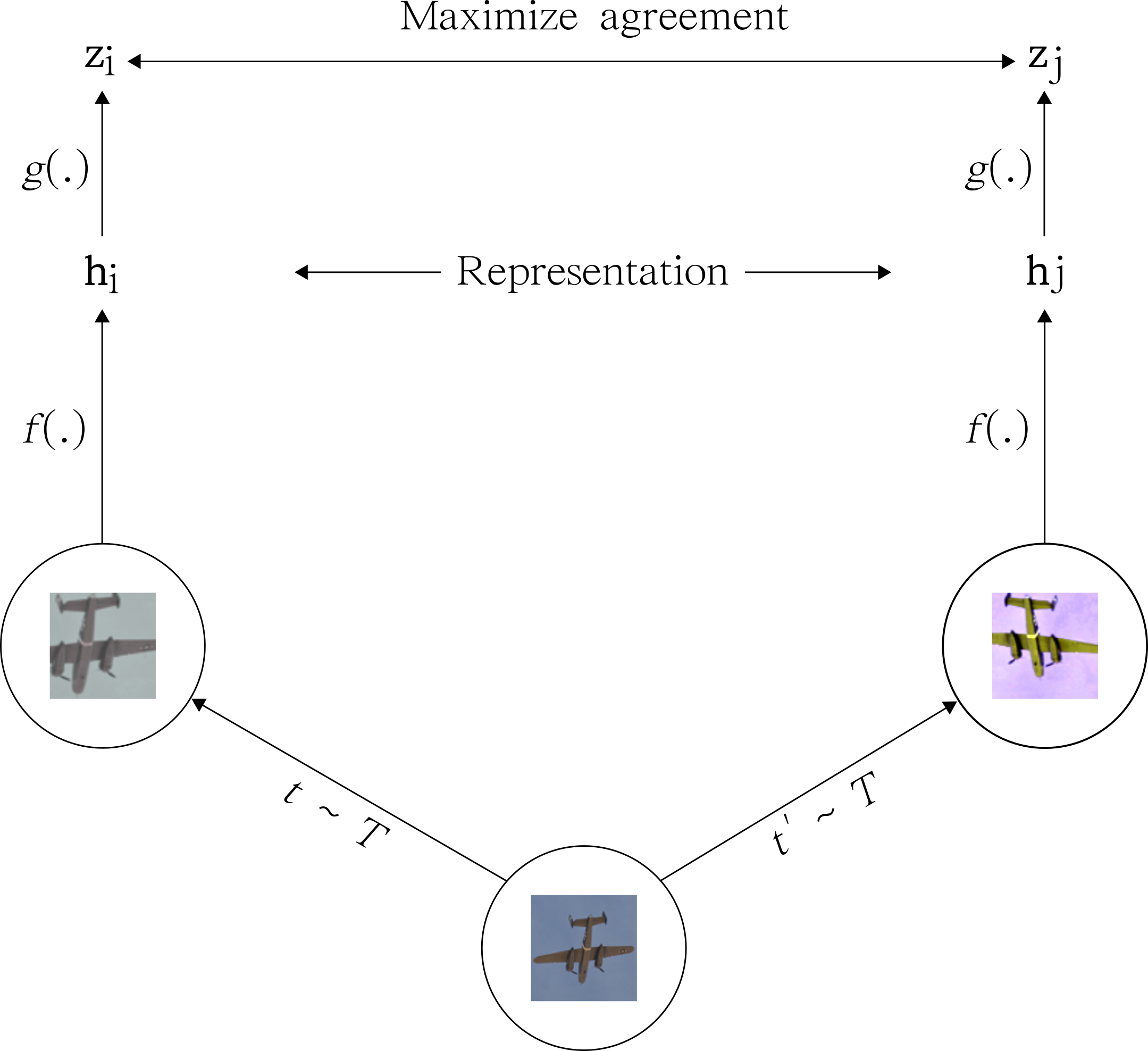
Credits: A Simple Framework for Contrastive Learning of Visual Representations
To understand SimCLR, let’s explore how it builds on the core components of the contrastive learning framework.
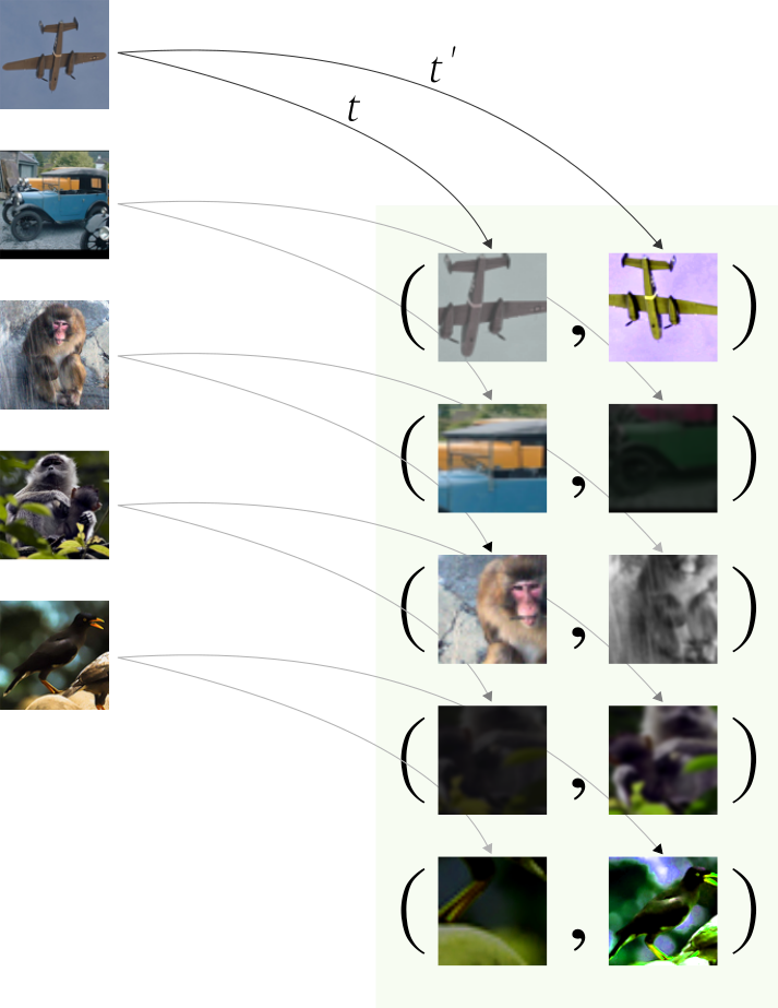
Given an input image, we create 2 correlated copies of it, by applying 2 separate data augmentation operators. The transformations include (1) random crop and resize, (2) random color distortions, and (3) random Gaussian blur.
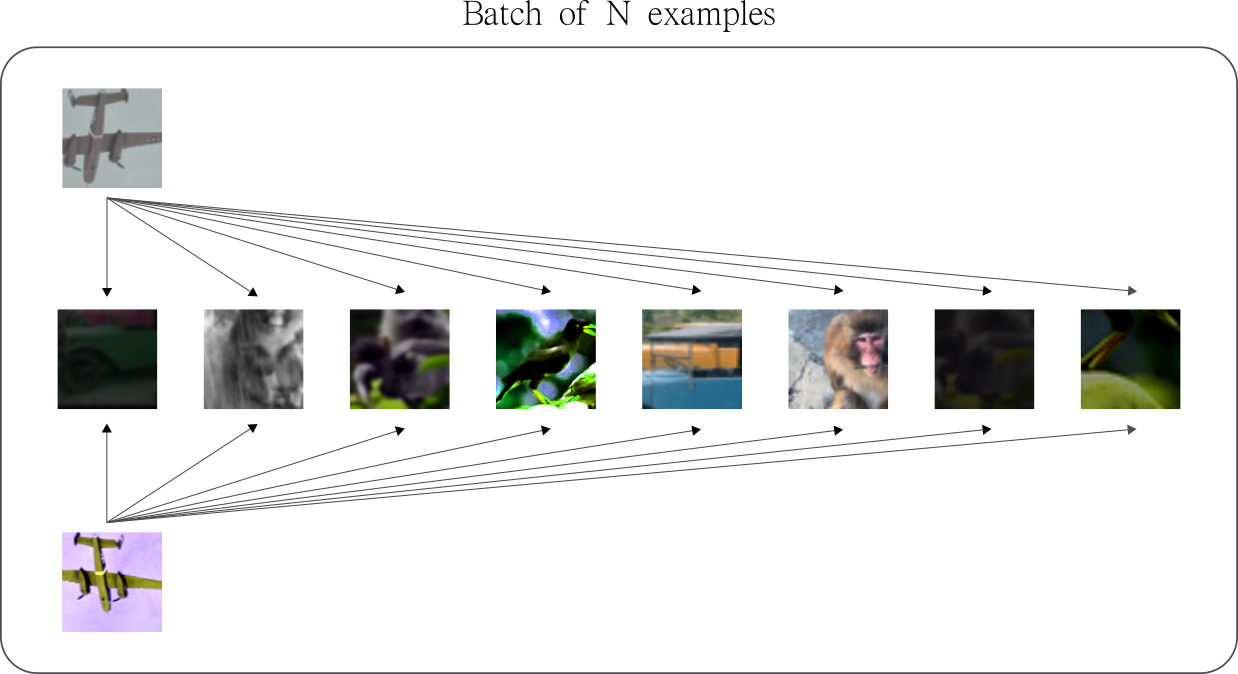
The order of the operations is kept fixed, but since each operation has its own uncertainty, it makes the resulting views visually different. Note that since we apply 2 distinct augmentation functions on the same image, if we sample 5 images, we end up with $2 \times 5 = 10$ augmented observations in the batch. See the visual concept below.
To maximize the number of negatives, the idea is to pair each image (indexed $i$) in the batch with all other images (indexed $j$). Note that we avoid pairing an observation $i$ with itself, and with its augmented version. As a result, for each image in the batch, we get $2 \times (N-1)$ negative pairs — where N is the batch size.
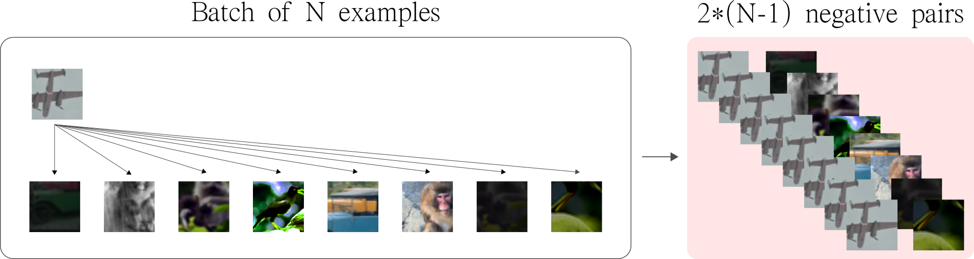
Note that the same method is applied to both augmented version of a given observation. This way, the number of negative pairs is increased even more.
Moreover, by arranging negative samples in this way, SimCLR has the advantage of not needing extra logic to mine negatives. To have an idea, recent implementations like PIRL and MOCO, uses a Memory Bank and a Queue, respectively, to store and sample large batches of negatives.
In fact, in the original implementation, SimCLR is trained with batch sizes as large as 8192. By following these ideas, this batch size produces 16382 negative examples per positive pair. In addition, the authors also showed that larger batches (hence more negatives) tend to produce better results.
SimCLR uses ResNet-50 as the main ConvNet backbone. The ResNet receives an augmented image of shape (224,224,3) and outputs a 2048-dimensional embedding vector $h$. Then, a projection head $g(.)$ is applied to the embedding vector $h$ which produces a final representation $z = g(h)$. The projection head $g(.)$ is a Multilayer Perceptron (MLP) with 2 dense layers. Both layers have 2048 units and the hidden layer has a non-linearity (ReLU) activation function.
For the similarity function, the authors use the cosine similarity. It measures the cosine of the angle between 2 non-zero vectors in a d-dimensional space. If the angle between 2 vectors is 0 degrees, the cosine similarity is 1. Otherwise, it outputs a number smaller than 1 all the way down to -1. Note that the contrastive learning loss operates on the latent space mapped by the projection head $g(.)$ — the $z$ embedding vectors.
Once the system is trained, we can through away the projection head $g(.)$ and use the representations $h$ (straight from the ResNet) to learn new downstream tasks.
Training and Evaluation
Once the components of the contrastive learning objective are in place, training the system is straight forward. You can have a look at my implementation here.
To train the model, I used the STL-10 dataset. It contains 10 different classes with a reasonable small number of observations per class. Most importantly, it contains a larger unsupervised set with 100000 unlabeled images – that is the bulk of images used for training.
For this implementation, I used a ResNet-18 as the ConvNet backbone. It receives images of shape (96,96,3), regular STL-10 dimensions, and outputs vector representations of size 512. The projection head $g(.)$ has 2 fully-connected layers. Each layer has 512 units and produces the final 64-dimensional feature representation $z$.
To train SimCLR, I took the train + unlabeled portions of the dataset – that gives a total of 105000 images.
After training, we need a way to evaluate the quality of the representations learned by SimCLR. One standard way is to use a linear evaluation protocol.
The idea is to train linear classifiers on fixed representations from the SimCLR encoder. To do that, we take the training data, pass it through the pre-trained SimCLR model, and store the output representations. Note that at this point, we do not need the projection head $g(.)$ anymore.
These fixed representations are then used to train a Logistic Regression model using the training labels as targets. Then, we can measure the testing accuracy, and use it as a measure of feature quality.
This Jupyter Notebook shows the evaluation protocol. Using the SimCLR fixed representations as training signals, we reach a test accuracy of 64%. To have an idea, performing PCA on the training data and keeping the most important principal components, we get a test accuracy of only 36%. This emphasizes the quality of the features leaned by SimCLR.
Some Final Remarks
The original SimCLR paper also provides other interesting results. These include:
- The results of unsupervised contrastive feature learning on semi-supervised benchmarks;
- Experiments and benefits of adding non-linear layers to the projection header;
- Experiments and benefits of using large batch sizes;
- The results of training large models with the contrastive objective;
- An ablation study on using a varied of stronger data augmentation methods for contrastive learning;
- The benefits of normalized embeddings for training contrastive learning-based models;
I encourage you to have a look at the paper for more details.
Thanks for reading!
Cite as:
@article{
  silva2020exploringsimclr,
  title={Exploring SimCLR: A Simple Framework for Contrastive Learning of Visual Representations},
  author={Silva, Thalles Santos},
  journal={https://sthalles.github.io},
  year={2020}
  url={https://sthalles.github.io/simple-self-supervised-learning/}
}