Understanding Linear Regression using the Singular Value Decomposition

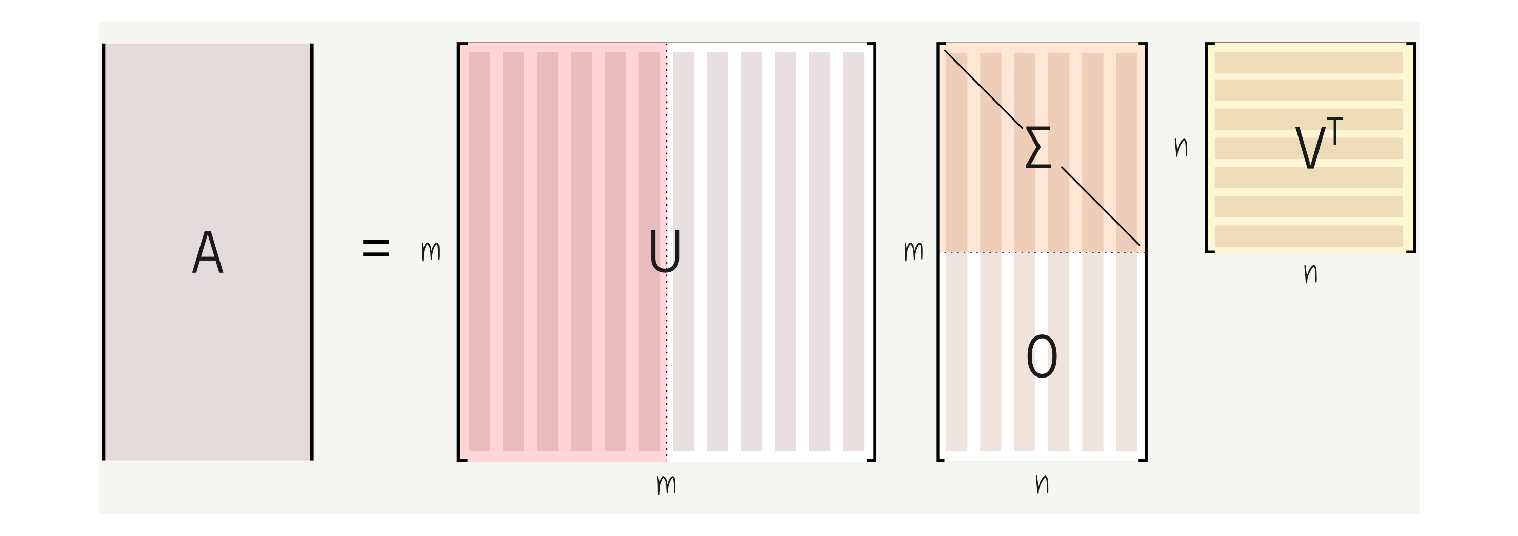
Introduction

It is very common to see blog posts and educational material explaining linear regression. In most cases, probably because of the big data and deep learning biases, most of these educational resources take the gradient descent approach to fit lines, planes, or hyperplanes to high dimensional data. In this post, we will also talk about solving linear regression problems but through a different perspective. Most specifically, we will talk about one of the most fundamental applications of linear algebra and how we can use it to solve regression problems. Yes, I am talking about the SVD or the Singular Value Decomposition. This computational tool is used as a basis to solve a myriad of problems, including dimensionality reduction, with PCA, and statistical learning using linear regression.

Linear Models and Systems of Linear Equations

Through the lens of linear algebra, a regression problem reduces to solving systems of linear equations of the form $Ax = b$. Here, $A$ and $b$ are known, and $x$ is the unknown. We can think of $x$ as our model. In other words, we want to solve the system for $x$, and hence, $x$ is the variable that relates the observations in $A$ to the measures in $b$.

Here, $A$ is a data matrix. We can think of the rows of $A$ as representing different instances of the same phenomenon. They can represent records for individual patients submitted to a hospital, records for different houses being sold, or pictures of different people’s faces. Complementary, we can view the columns of the matrix $A$ as recording different characteristics of each instance in the rows of $A$. In a patient hospital example, such features might include the blood pressure when he/she arrived at the hospital or if the patient has had a surgical procedure or not.

Also, note that the matrix $A$ might have different shapes. First, $A$ could be a square matrix. Yes, it is very unlikely (for the situations we usually encounter in data science) but otherwise possible.

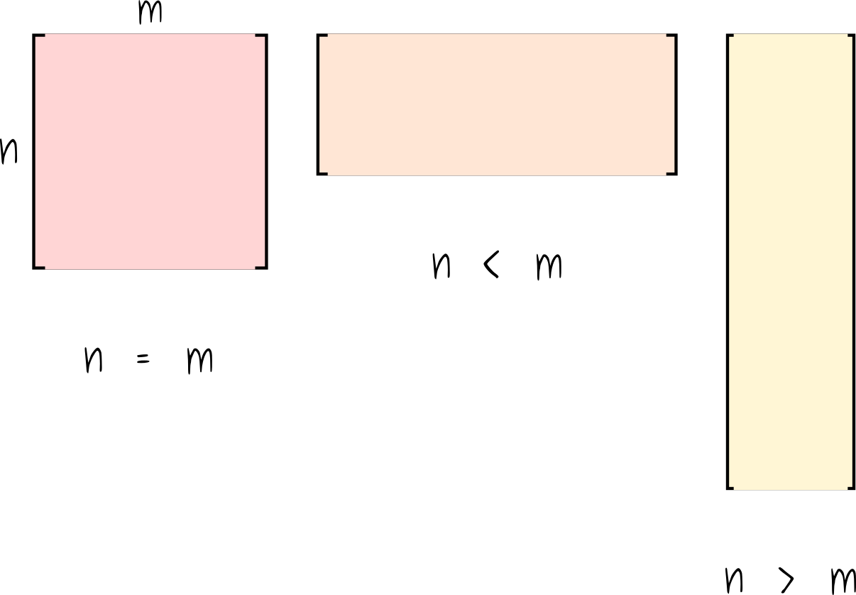
Second, $A$ could have more columns than rows. In this scenario, $A$ would have a short and wide shape. And lastly, (and that is the most usual case in data science), the matrix $A$ assumes the form of a tall and skinny matrix, with many more rows than columns.

But why should I care for the shape of the matrix $A$?

Interestingly, the shape of $A$ will dictates whether the linear system of equations has a solution, has infinitely many solutions, or does not have a solution at all.

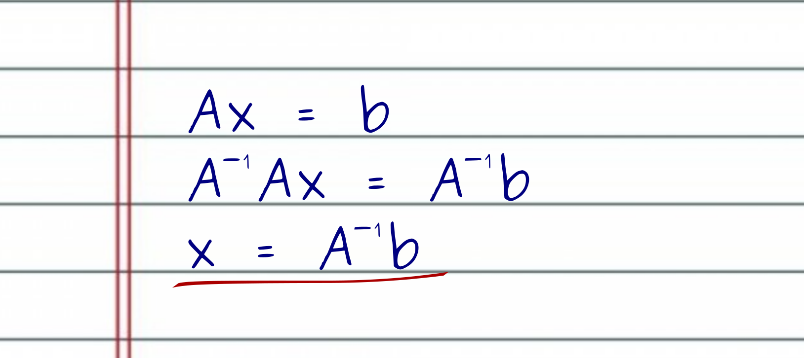
Let’s start with the boring case. If the matrix is squared (number of rows equals the number of columns) and it is invertible, meaning that the matrix $A$ has full rank (all columns are linearly independent), that pretty solves the problem.

However, if the matrix has more columns than it has rows, we are likely dealing with the case where there are infinitely many solutions. To visualize this curious scenario, picture a $3 \times 6$ matrix, i.e., 3 rows and 6 columns. We can think of it as having a 3D space and 6 different vectors that we can use to span the 3D space. However, to span a 3D space, we only need 3 linearly independent vectors, but we have 6! This leaves 3 dependent vectors that can be used to formulate infinitely many solutions.

Finally, by analogy, if we have a matrix $A$ with more rows than columns, we can view it as trying to span a very high-dimensional space with fewer vectors than we would need. For instance, picture a matrix with 6 rows and 2 columns. Here, we have a 6D space, but we only got 2 vectors to span it. It does not matter how much we try it, in the best case, we can only span a plane on 6D. And that is crucial because we only have a solution to $Ax = b$ if the vector $b$ is in the column space of $A$. But here, the column space of $A$ spans 2D subspace (a plane) on a much larger 6D space. This makes the probability of the vector $b$ to be in the subspace spanned by the columns of $A$ improbable.

To visualize how unlikely it is, picture a 3D space and a subspace spanned by two vectors (a plane in 3D). Now, imagine you choose 3 values at random. This will give you a point on the 3D space. Now, ask yourself: what is the probability that my randomly chosen point will be on the plane?

Nonetheless, in situations where we do not have a solution for a linear system of equations $Ax = b$ (or we have infinitely many solutions), we still want to do our best. And to do this, we need to find the best approximate solution. Here is where the SVD kicks in.

A Short Intro to the SVD

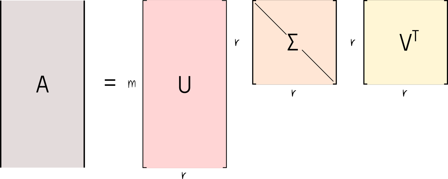
The main idea of the singular value decomposition, or SVD, is that we can decompose a matrix $A$, of any shape, into the product of 3 other matrices.

Here, $U$ is an $m \times m$ square matrix, $\Sigma$ is a rectangular matrix of shape $m \times n$, and $V^T$ is a square matrix and has shape $n \times n$.

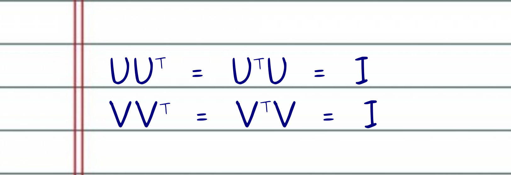
The matrices $U$ and $V^T$ have a very special property. They are unitary matrices. One of the main benefits of having unitary matrices like $U$ and $V^T$ is that if we multiply one of these matrices by its transpose (or the other way around), the result equals the identity matrix.

On the other hand, the matrix $\Sigma$ is diagonal, and it stores non-negative singular values ordered by relevance.

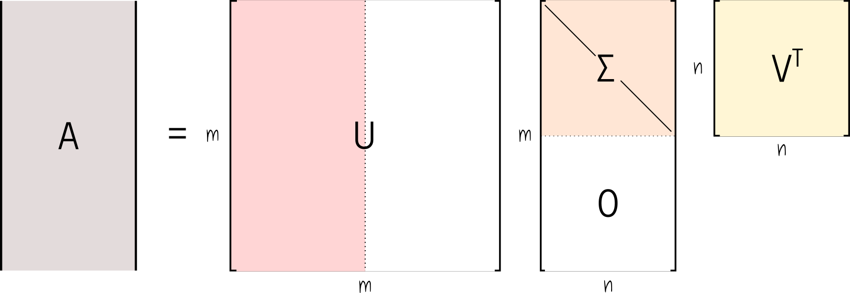
Note that, since the $\Sigma$ matrix is diagonal, only the first $n$ row diagonal values are worth keeping. Indeed the last $n$ rows of $\Sigma$ are filled with 0s. For this reason, it is very common to keep only the first $r \times r$ non-negative diagonal values of $\Sigma$, along with the corresponding $r$ columns and rows of $U$ and $V^T$ respectively. Note that $r = min(m, n)$. This is commonly referred to as the economy (or compact) SVD, and from this point on, we will assume the matrices $U$, $\Sigma$, and $V^T$ are derived from the economy procedure.

Quick note, it is very common to also truncate the SVD based on some criteria. Under some assumptions, it is possible to find an optimal threshold for suppressing some of the singular values with small magnitudes.

It is important to note that the economy SVD produces a change in the shape of the matrices $U$ and $\Sigma$ (if one of the diagonal values of $\Sigma$ is zero, $V^T$ also suffers a shape change). If the diagonal values of $\Sigma$ are all positives, thus $r = n$, we discard the right half of the $U$ matrix (the orthogonal complement of $U$), which gives $U$ a rectangular $m \times r$ shape. More critical, $U$, and possibly $V^T$, are now semi-unitary matrices, which means that only $U^TU = V^TV = I$.

The SVD provides a basis that allows us to reconstruct the input signal in terms of low-rank matrix approximations. Let me be more clear. If we combine each column of $U$ with the corresponding row of $V^T$, and scale the resulting matrix by the corresponding $\sigma$ value, we will get the best rank-1 approximation of $A$ in terms of least squares.

And as we continue combining the columns of $U$ with rows of $V^T$, scaled by the corresponding $\sigma$, we get the next best rank-i approximation of the data matrix $A$. Indeed, that is another excellent application of the SVD–data compression. But that is a subject for another writing.

As we said before, the problem of working with a non-square matrix $A$ is that we cannot invert it. And that is the main reason why we cannot solve the system of equations as we would for a square matrix $A$. However, if we cannot invert the matrix $A$, I invite you to ask yourself the following question.

What would be the best matrix $A^+$ that, when multiplied by $A$, would come as close as possible to identity matrix $I$?

The answer to this question solves the problem of finding the best possible solution when the system of equations has infinitely many solutions or no solution at all. Luckily, the answer also lies in the SVD.

If we know that the SVD always exists (for matrices of any shape), and by combining the columns of $U$, the rows of $V^T$, and the singular values $\sigma$, we can reconstruct the original input matrix nearly perfectly, what happens if we try to invert the SVD?

Let me spoil it with no further ado. It turns out that the best matrix $A^+$ that approximately solves the question $A^+A \approx I$ is the inverse of the SVD. In other words, the best approximation for $A^{-1}$ is $SVD^{-1}$. Let’s follow the math.

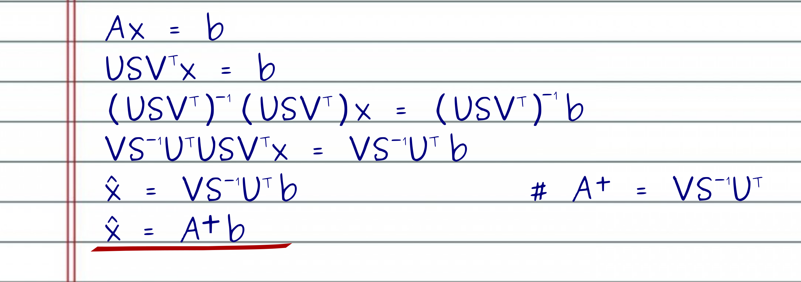
First, we compute the SVD of $A$ and get the matrices $USV^T$. To solve the system of equations for $x$, I need to multiply both sides of the equation by the inverse of the SVD matrices. Luckily now, it is very easy to invert each one of the 3 SVD matrices. To invert the product of the 3 matrices $USV^T$, I take the product of the inverse matrices in reverse order!

After inverting the matrices, if we look closely at the left-hand side, we can see that most matrices will cancel like crazy, leaving us with the best approximate solution for $\hat{x}$. Note that since the matrix $U$ is semi-unitary, only $U^TU = I$ holds. Moreover, if (and we assume that) all the singular values are non-negative, then $V^T$ continuous to be a unitary matrix. Hence, to invert $U$ and $V^T$, we just multiply each one by their transpose, i.e., $U^TU = I$ and $VV^T = I$.

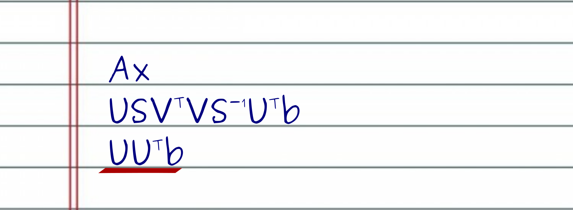
If we go further and substitute our best solution $\hat{x}$ into $A\hat{x}$, we will see that most of the matrices cancel each other as well, until we reach $UU^T$. As we said before, $U$ is semi-unitary, and $UU^T$ is not the identity matrix. Instead, $UU^T$ is the projection of $b$ onto the subspace spanned by the columns of $U$ (hence columns of $A$), which is the best approximate solution in terms of least squares, i.e., we found the least squares solution $\hat{x} = minimum(\left | A\hat{x}-b \right |_2)$.

Note that if $A$ has more columns than rows and infinitely many solutions, the SVD picks the solution with the minimum 2-norm, i.e., $\hat{x} = minimum(\left | \hat{x} \right |_2)$.

Linear Regression with the SDV

Once we have established the required SVD jargon, we can use it to find approximate solutions for real-world problems. In this example, I am going to use the Boston house-prices dataset. The house-prices data matrix $A$ contains 506 rows (representing individual houses), and 13 columns (each describing a different characteristic of the houses). Some of these 13 features include:

• Per capita crime rate by town
• The average number of rooms per dwelling
• Weighted distances to five Boston employment centers

You can see the full description here.

We want to predict the median value home price in $1000’s. These measurements are real values ranging from 5 to 50, and they represent the $b$ vector in our system of equations $Ax = b$.

As usual, the matrix has many more rows than columns. This means that we cannot invert $A$ to find the solution to $Ax = b$. Also, it drastically reduces the possibilities of finding a solution. Indeed, such a solution would only be possible if $b$ is a linear combination of the columns of $A$. However, using the SVD, we will be able to derive the pseudo-inverse $A^+$, to find the best approximate solution in terms of least squares – which is the projection of the vector $b$ onto the subspace spanned by the columns of $A$.

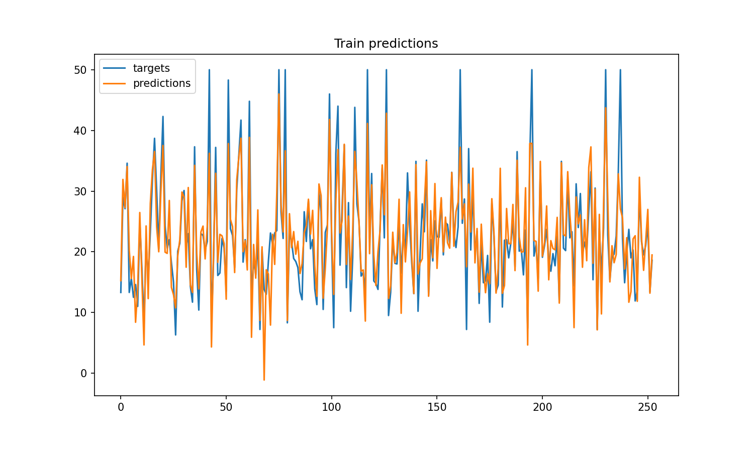
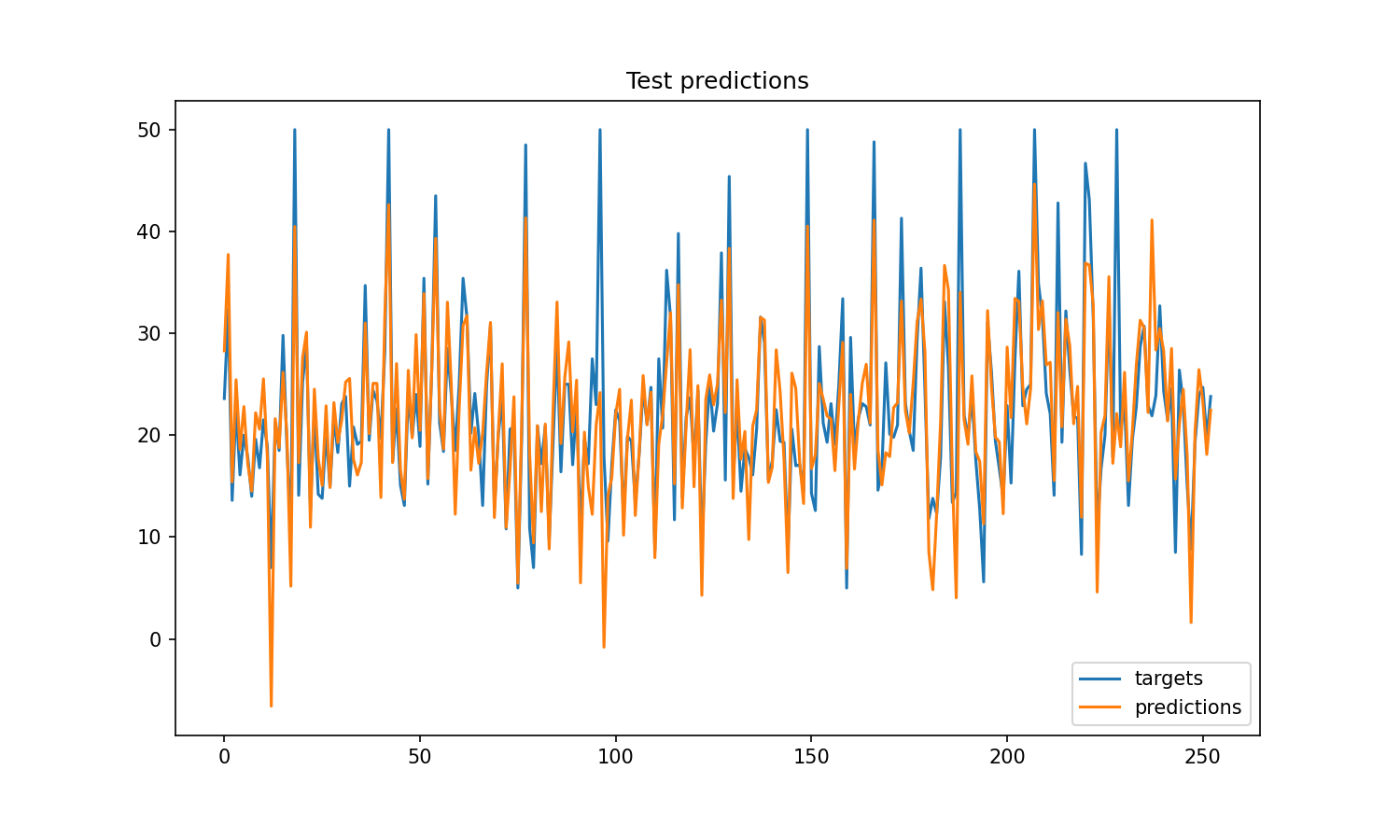
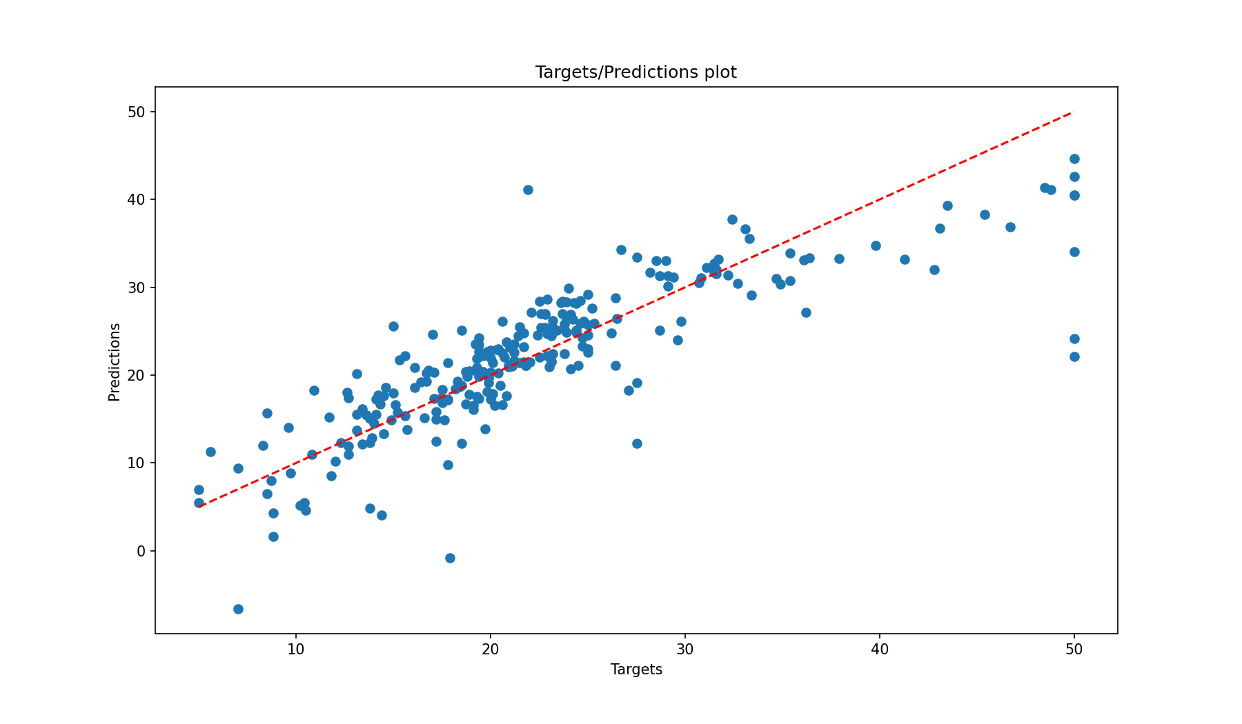
The code is very simple to follow, and the results are excellent. Indeed, they are the best possible for a linear model.

One quick note, look at line 9 of the python code above. At this line, I appended a column full of 1s to the data matrix $A$. This column will allow the linear model to learn a bias vector that will add an offset to the hyperplane so that it does not cross the origin.

Take a look at the train and test results below.

Thanks for reading!

Cite as:

@article{
  silva2020svdregression,
  title={Understanding Linear Regression using the Singular Value Decomposition},
  author={Silva, Thalles Santos},
  journal={https://sthalles.github.io},
  year={2020}
  url={https://sthalles.github.io/svd-for-regression/}
}